NaN Rendering Semantics and Their Performance Cost¶

Abstract — Missing values in scientific data almost always enter the plotting pipeline as IEEE-754 NaN: a sensor dropping offline, a division by zero, a failed interpolation/extrapolation step, an explicit hole from an upstream pipeline. A renderer facing NaN has only three semantic choices: split the polyline at the gap (matplotlib's choice), skip the sample and join the two sides, or draw it as 0; the three mean completely different things visually. Reading QWT7's qwt_point_mapper.cpp and qwt_plot_curve.cpp line by line gives the exact output semantics on NaN data of five paint attributes (ClipPolygons without filtering / FilterPoints / FilterPointsAggressive / FilterPointsPixel / FilterPointsLTTB): QWT7 implements skip semantics. Every Lines-family path outputs a single continuous polyline, and NaN runs are "bridged" over by a chord instead of being split. A 3090-group polygon-hash comparison between a line-by-line Python reimplementation and the real library (100% agreement) and a per-pixel visual scan of 960×560 offscreen renders (0.23%–3.80% of pixels differ from the ideal split reference) confirm this jointly. On the performance side, the boundingRect cold scan is a single $O(n)$ sequential read, about 12–22 ms for one million points; the SIMD argmin/argmax path degrades globally to scalar as soon as any NaN appears, but in frame-level measurements this "cliff" is masked by the data-reduction gains and the rasterization-dominant term (delta = −0.29 at 100k points, delta = +0.03 at 1M points, consistent with the nanperf example's conclusions).

Abstract — Core conclusions

QWT7's NaN semantics are skip-not-split: in the semantics matrix of 14 NaN patterns × 5 paint attributes, every Lines-family path produces exactly 1 bridging chord for every interior NaN run (run pattern: 3 gaps → 3 bridging chords, no exception among the five modes); only per-sample styles like Dots / Sticks are naturally correct.

Semantic-reimplementation cross-validation: the line-by-line Python reimplementation and the real qwtplot.dll output agree on 3090/3090 (100%) polygon hashes across 15 directed cases + 250 random cases × 2 canvases × 6 paths; 90 directed-case groups match bit-for-bit vertex by vertex.

Visual artifacts (per-pixel comparison against the ideal rendering of "break at NaN, everything else unchanged", 960×560): among the interior-gap patterns, FilterPointsAggressive is closest to the ideal (0.23%–1.05% differing pixels) and FilterPointsLTTB deviates the most (2.50%–3.80%), of which about 2.7 percentage points come from bucket-boundary reshuffling rather than bridging.

Performance: for the 1M-point Middle case, frame time (min-of-7) decreases overall as the NaN ratio goes from 0% to 50% (individual 1%/5% cells rebound within measurement noise): no-filter 173.7→86.5 ms, FilterPointsLTTB 26.3→13.1 ms; boundingRect cold scan 21.7→11.5 ms; all-NaN data takes only 0.6–1.7 ms per frame, the canvas is blank, and the axes fall back to 0–1000.

Beyond the first item of the failure list there are two measured traps, both on the LTTB MinMax-bucket raw-pointer path (the implementation behind FilterPointsLTTB at the time of writing; moved to FilterPointsMinMaxLTTB in v7.5.0): the pre-scan checks only y, so a sample whose x is NaN and y is finite, if it happens to be a bucket extremum, lands in canvas column 0 via qRound(NaN)==0 (measured, MSVC x64 + Qt 5.15) and forms a spurious spike; and +Inf can pass through the isnan-only pre-scan into the SIMD path, producing INT_MIN pixel coordinates. Both are fixed in v7.5.0 (see the Section 5 update record). The raw-pointer branch of the true LTTB introduced in v7.5.0 (the default FilterPointsLTTB) still uses the y-only isnan test, so x and Inf must be cleaned before it as well.

1. Introduction: where NaN comes from and what the renderer should do¶

1.1 Three sources¶

NaN in engineering data is a routine encoding, not an anomaly. A sensor drops offline within a sampling interval and the acquisition side writes qQNaN() as a placeholder; a physical quantity is divided by a denominator crossing zero, and IEEE-754 dictates the result is ±Inf or NaN; a data-cleaning pipeline replaces outliers with explicit holes, and downstream NaN means "no measurement here". What the three sources have in common: NaN carries positional information (the $i$-th sample is missing) and missingness information (the value is unknown), and any rendering that treats NaN as a numeric value loses both at once.

1.2 Formalizing the rendering semantics¶

Let the sample sequence be $P=\{(x_i,y_i)\}_{i=0}^{N-1}$, and denote the maximal contiguous runs of finite samples by $S_1,S_2,\dots,S_k$. The ideal split semantics is defined by: the rendering operator $\mathcal{R}$ satisfies

\[ \mathcal{R}_{\text{ideal}}(P) = \bigcup_{j=1}^{k} \mathcal{R}(S_j) \]

that is, each contiguous run renders independently, with no connecting primitive between runs; a missing run leaves a blank on the canvas. This is the behavior of matplotlib's polylines and the eye's intuitive reading of "missing data". The skip semantics instead deletes the NaN samples from the sequence and renders the whole:

\[ \mathcal{R}_{\text{skip}}(P) = \mathcal{R}\left( \bigcup_{j} S_j \text{(concatenated in original order)} \right) \]

Concatenation introduces a bridging chord between adjacent runs: the segment connecting the last point of $S_j$ to the first point of $S_{j+1}$, which has no basis in the data at all. The draw-as-zero semantics (treating NaN as 0) destroys even the positional information and is out of scope. The difference among the three semantics becomes more glaring the larger the $y$ values differ across a gap and the wider the gap: a bridging chord can span half the canvas, welding two unrelated signals together.

QWT7's choice is the skip semantics. The documentation does not make this claim; the five mapping paths of src/plot/qwt_point_mapper.cpp show it line by line: every path's main loop is if (qwt_is_nan_or_inf(sample)) continue;, the sample is dropped and vertices keep appending to the same QPolygonF. Section 3 gives the per-path evidence, and Section 4 measures how many pixels the bridging chords get wrong.

1.3 Beyond polylines: NaN semantics in the other primitives¶

The same isfinite check carries different semantics in the other branches of the pipeline; reading them side by side helps see that "skip" is a general principle in QWT rather than a polyline special case. QwtPlotSpectrogram renders NaN cells as transparent pixels (writes 0 when hasGaps && qwt_is_nan_or_inf(value), qwt_plot_spectrogram.cpp lines 598/620; the earlier bit-level qwtIsNaN has been removed and the current predicate intercepts Inf as well), and provides the QwtRasterData::WithoutGaps flag so gap-free data skips the per-cell check. In raster semantics "gap means transparent" holds naturally because pixels have no connection relation. The CONREC contour algorithm detects NaN via an accumulated sum (the cell is skipped when qwt_is_nan_or_inf(zSum), qwt_raster_data.cpp line 373, again intercepting Inf too), exploiting NaN's absorption law under addition. For the scatter and symbol paths (qwtToPointsFiltered, drawSymbols), skipping NaN is the correct semantics, for the same reason as Dots/Sticks. Only primitives with a notion of "connection", namely polylines and steps, expose the divergence between skip and split, which is what this report examines.

1.4 Division of labor with the existing documentation¶

The use guide NaN Data Handling answers "how to configure and how to generate the data"; Sections 5.3 and 5.4 of Curve Downsampling already give the structure diagrams of the MinMax bucket's three paths and the NaN pre-scan. This report takes the principles view: the propagation of IEEE-754 comparison semantics through every layer of the rendering pipeline is written as verifiable propositions, with three sets of numbers (the semantics matrix, the visual artifacts, and the performance cost) backed by reproducible experiments.

2. IEEE-754 comparison semantics and pipeline propagation¶

2.1 Ordered predicates: NaN is "invisible" to comparisons¶

IEEE-754 dictates that every comparison except != returns false for NaN: $\mathrm{NaN} < x$, $\mathrm{NaN} > x$, $\mathrm{NaN} \le x$ are all false. This rule propagates through the rendering pipeline layer by layer, with different effects at each:

boundingRect layer (qwtBoundingRectT in src/core/qwt_series_data.cpp, lines 217–261): the Qwt 6 era relied on qMin/qMax to extend the bounds; NaN made all comparisons false, so the bounds either stopped extending or were polluted into invalid values. QWT7 switched to an explicit isSampleNanOrInf(sample) skip (one continue in each of the two loops, lines 236–237 and 248–249), and the bounding rectangle is determined by finite samples only. An all-NaN sequence returns the invalid rectangle QRectF(1,1,-2,-2) (measured: boundingRect_allNan_valid=0, x=1, width=-2).
Autoscaling layer (two sites, different mechanisms): QwtPlot::rescaleAxes() (src/plot/qwt_plot.cpp lines 1908–1911) checks the finiteness of all four sides with qwt_is_nan_or_inf before merging bounding rectangles; the autoscaling at replot time goes through QwtPlot::updateAxes() (src/plot/qwt_plot_axis.cpp lines 865–869), which merges intervals only when width()/height() >= 0. The invalid rectangle (1,1,-2,-2) of an all-NaN sequence has negative width and height and is skipped entirely, the axis interval stays invalid and falls back to the AxisData default range 0–1000 (same file, lines 43–44; measured autoscale_allNan_x_upper=1000), and nothing is drawn on the canvas.
SIMD argmin/argmax layer (the AVX2 kernel lives in its own file since v7.5.1, src/core/qwt_simd_argminmax_avx2.cpp, main loop lines 64–79; dispatch and the NaN fallback in src/core/qwt_simd_argminmax.cpp): comparisons use the ordered predicates _CMP_LT_OQ / _CMP_GT_OQ (lines 72/76); NaN can never win a comparison and never enters the index vectors; the horizontal reduction and the scalar tail likewise use ordered comparisons. So "NaN is ignored naturally" holds at the level of value semantics.

The NaN-detection predicates used by the layers are not uniform; this table is the index for the failure list later:

Layer	Predicate	What is checked	Intercepts Inf?
`qwtBoundingRectT` / curve styles / Quad / Pixel / generic bucket path	`qwt_is_nan_or_inf` = `!isfinite`	both x and y coordinates	yes
MinMax pre-scan (lines 725–731, since v7.5.0)	`!std::isfinite`	y only	yes (for y only; x is not checked)
MinMax scalar bucket loop (lines 680–687, since v7.5.0)	`!std::isfinite`	both x and y coordinates	yes
True-LTTB raw-pointer branch (`qwtLttbReduce`'s `mapSample`, lines 915–922)	`std::isnan`	y only (x is not checked)	no (±Inf and non-finite x both pass)
`qwtSimdArgMinMax` fallback (lines 170–172)	`std::isnan(result.minVal/maxVal)`	reduction result	partially (returns the sentinel `{0,0,DBL_MAX,-DBL_MAX}` when the result is still NaN)

Predicate strength decreases from left to right: the dual-coordinate isfinite is the strongest form, the single-coordinate isnan the weakest. Items 3 and 4 of the Section 5 list were direct consequences of the original first two rows (the MinMax side has been completed in v7.5.0); the same single-coordinate isnan left in the true-LTTB raw-pointer branch continues that history, and cleaning per Section 6.4 is still required before using it.

2.2 Index semantics are unreliable: why the pre-scan is still needed¶

Correct value semantics does not mean correct (value, index) pairs. The instruction maintaining the running value in the AVX2 main loop is _mm256_min_pd(minVec, vals), and MINPD returns the second operand when either operand is NaN: if a lane reads NaN, that lane's running value becomes NaN; on the next round vals < NaN is false, so the index vector is not updated, but the running value is restored to the new value by _mm256_min_pd(NaN, vals), a "value is new, index is old" mismatch, and the emitted extremum welds one sample's $y$ to another sample's $x$. This is exactly why qwtMinMaxBucketReduce runs a non-finite y pre-scan before the raw-pointer fast path (qwt_point_mapper.cpp lines 725–731): as soon as the pre-scan finds any non-finite y, the whole range switches to the scalar bucket loop (reduceBucketScalar, lines 671–716; the whole-range call at lines 765–769), trading one $O(n)$ sequential read for the per-bucket branches and the mismatch risk; non-finite x values are not part of the pre-scan and are instead caught by the SIMD path's per-bucket post-check (lines 747–753). The pre-scan short-circuits with a break: data free of non-finite y pays the full $O(n)$ cost, data that hits pays only up to the first hit, an asymmetry visible in the frame-time curves of Section 4.4.

Walk through the mismatch with an 8-sample bucket (single-lane view, min side):

Round	vals	cmp = vals < minVec (LT_OQ)	minVec (after MINPD)	minIdx
0	5.0	true (5 < DBL_MAX)	5.0	0
1	NaN	false	NaN (MINPD returns the second operand)	0
2	3.0	false (3 < NaN is false!)	3.0	0 ← should be 2
3	4.0	false	3.0	0

Round 2's true minimum 3.0 enters the running value but loses its own index because the ordered comparison against NaN is false; at the end of the bucket the output is (value=3.0, index=0), while the sample at index 0 has value 5.0. In the SIMD branch of qwtMinMaxBucketReduce this mismatch becomes a direct mismatch between raw.x[minI] and r.minVal, a data point that does not exist geometrically. The pre-scan changes the whole path from "defend in every bucket" to "decide once, reroute the whole range", a classic engineering trade of one sequential scan for the branches of the hot loop.

flowchart TD
    A["Bucket loop start<br/>numBuckets = max(2, 2W)"] --> B{"Linear mapping and<br/>raw Y pointer extractable?"}
    B -->|"no"| C["Generic path<br/>sample(i) per point<br/>isfinite check on both coordinates"]
    B -->|"yes"| D["Non-finite y pre-scan<br/>i in visFrom..visTo<br/>!isfinite(raw.y[i]), short-circuit break"]
    D --> E{"Any non-finite y in the range?"}
    E -->|"no"| F["SIMD fast path<br/>qwtSimdArgMinMax once per bucket<br/>+ per-bucket x post-check"]
    E -->|"yes"| G["Scalar fast path<br/>raw pointers + !isfinite on both coordinates<br/>non-finite x and y samples skipped"]
    F --> H["1-2 extreme points per bucket<br/>all-NaN buckets emit nothing"]
    G --> H
    C --> H

2.3 Rounding functions: where NaN and Inf finally land¶

The mapped pixel coordinates pass through rounding functions, where NaN/Inf receive definite (but unexpected) integer values. Qt 5.15 implements qRound(double) as d >= 0 ? int(d+0.5) : int(d - double(int(d-1)) + 0.5) + int(d-1); on MSVC x64, int(NaN) goes through cvttsd2si and yields the "integer indefinite value" INT_MIN, and adding two INT_MINs wraps around to 0 in int32. Measured (nan_mapper_check probes):

Input	`qRound` result (MSVC x64, Qt 5.15.16)	Rendering consequence
`NaN`	`0`	spurious vertex lands in canvas column 0
`+Inf`	`-2147483648` (`INT_MIN`)	flies off the canvas, clipped away by `ClipPolygons`
`-Inf`	`0`	spurious vertex lands in canvas column 0

The floating-point rounding qwtRoundValueF (floor(v+0.5) / ceil(v-0.5)) instead lets NaN pass through unchanged: QPolygonF keeps a (NaN, NaN) vertex. These two tables are the arithmetic roots of two traps in the Section 5 failure list.

flowchart TD
    A["QwtSeriesData&lt;QPointF&gt;<br/>with NaN/Inf samples"] --> B["qwtBoundingRectT<br/>isfinite skip; all-NaN yields an invalid rect"]
    B --> C{"Any finite samples in the sequence?"}
    C -->|"no"| D["Axes fall back to 0..1000<br/>canvas blank"]
    C -->|"yes"| E["drawLines / drawSteps / drawDots / drawSticks<br/>each skips NaN"]
    E --> F{"QwtPointMapper flag priority<br/>Pixel &gt; LTTB &gt; MinMax &gt; Quad &gt; WeedOut"}
    F --> G["qwtPixelColumnReduce<br/>continue skips; empty columns emit nothing"]
    F --> H["qwtMinMaxBucketReduce<br/>non-finite y pre-scan -&gt; SIMD (+x post-check) / scalar / generic"]
    F --> I["qwtMapPointsQuad<br/>first-non-NaN scan + continue"]
    F --> J["qwtToPolylineFiltered / qwtToPoints<br/>continue skips"]
    G --> K["Single QPolygonF<br/>NaN runs spanned by bridging chords"]
    H --> K
    I --> K
    J --> K

3. NaN handling in the five paths, one by one¶

3.0 From user attributes to mapper flags¶

QwtPlotCurve::drawLines (qwt_plot_curve.cpp lines 583–698) translates user-level attributes into mapper flags: FilterPoints → WeedOutPoints; FilterPointsAggressive → WeedOutIntermediatePoints (only when integer alignment doAlign is true, lines 609–612) + WeedOutPoints; FilterPointsPixel → PixelColumnReduce; FilterPointsLTTB → LTTBReduce (true LTTB since v7.5.0; up to v7.4.2 it mapped to MinMaxReduce); FilterPointsMinMaxLTTB → MinMaxReduce (lines 614–619). The priority in toPolygonF is PixelColumnReduce > LTTBReduce > MinMaxReduce > WeedOutIntermediatePoints > WeedOutPoints (qwt_point_mapper.cpp lines 1502–1503). The analysis below follows this order; the lttb/lttbgen modes of Section 3.5 and the Section 3.8 semantics matrix denote the MinMax bucket path (all NaN measurements in this article were made with it; the harness kept the mode names), and the mode names follow the nanperf example's FilterModes.h.

3.1 No filtering (ClipPolygons only): `qwtToPoints`¶

qwtToPoints (lines 1135–1194) is the most naive path: iterate over [from,to], continue when qwt_is_nan_or_inf(sample) is true, otherwise transform, round per RoundPoints, and append. The invalid-bounding-rect branch does a single resize(numPoints) after the appending (line 1190; the comment on the line above, line 1189, explicitly says that after adding the NaN check this must be resized too). Semantics: remove NaN, keep order, one polyline; the bridging-chord count equals the number of interior NaN runs. All-NaN input yields an empty polygon.

3.2 FilterPoints: `qwtToPolylineFiltered`¶

qwtToPolylineFiltered (lines 1222–1268) first scans for the first non-NaN sample:

realFrom = from; sample0 = series->sample(from)
while (realFrom < to && qwt_is_nan_or_inf(sample0)): realFrom++, sample0 = series->sample(realFrom)
if realFrom >= to && qwt_is_nan_or_inf(sample0): return empty polygon   # all-NaN early exit (since v7.5.0)
points[0] = round(transform(sample0))          # a finite sample, no further check needed
for i = realFrom+1 .. to:
    if qwt_is_nan_or_inf(sample(i)): continue  # skip, do not split
    p = round(transform(sample(i)))
    if points[pos] != p: points[++pos] = p     # dedupe consecutive pixel duplicates

At the time of writing there was no all-NaN early exit here, unlike the Quad path: if the entire sequence is NaN, the loop stops at realFrom == to and points[0] is built from the last sample; with finite x and NaN y this yields a single-vertex polygon like (899, NaN) (semantics matrix, all row: points mode, 1 vertex, 1 garbage coordinate). A single-vertex polyline draws nothing under the rasterizer, so the all row of the visual scan differs by 0, but the polygon is non-empty: item 5 of the Section 5 list. Since v7.5.0 the same all-NaN early exit as in the Quad path has been added (lines 1245–1248): all-NaN input returns an empty polygon and the "empty polygon == no data" convention holds again; the 1 vertex in the matrix's all row is a pre-fix snapshot value (regression test tests/nan_curve_test/filterPoints_allNan_emptyPolygon).

3.3 FilterPointsAggressive: `qwtMapPointsQuad`¶

Two-pass quad merge (lines 218–345): the first pass skips NaN over the sequence and scans for the first non-NaN sample, and does have an all-NaN early exit (lines 235–236, if (realFrom >= to && qwt_is_nan_or_inf(sample0)) return polyline;); the second pass merges again on the integer polygon. NaN samples are removed by continue in the first pass, so the extreme statistics within a pixel column/row see only finite samples; the connection across a gap falls out naturally from the polyline after both merge passes, still a bridge. The orientation probe qwtProbeOrientation (lines 82–110) classifies a sequence whose x contains NaN as Vertical because (NaN > prev) != isIncreasing, changing the order of the two merge passes: in sweep B, the aggressive frame times of the xynan/xyinter cases (3.57/3.60 ms) are about 24% lower than middle (4.70 ms), the source is the change in output vertex count caused by this path flip, not less work.

3.4 FilterPointsPixel: `qwtPixelColumnReduce`¶

Pixel-column bucketing (lines 422–535): the main loop continues past NaN and then accumulates first/min/max/last per column; in the output phase, columns with count == 0 are not emitted at all. So the columns corresponding to a NaN run are empty columns, and the polyline connects the column left-adjacent to the gap directly to the right-adjacent column; the bridging chord here appears as a long chord spanning the empty columns. The sub-pixel placement within a column (+0.2/+0.25/+0.75/+0.8, lines 508–531) matches what Section 4.4 of Curve Downsampling describes; NaN does not change the placement rules, only which columns are non-empty.

# NaN behavior of qwtPixelColumnReduce (linear fast path, lines 451-471)
visFrom, visTo = findVisibleRange(xMap, series, from, to)   # x-NaN can make it fall back to the full range
bins[col] = {firstY, minY, maxY, lastY, count} for col in 0..W-1
for i in visFrom .. visTo:
    if qwt_is_nan_or_inf(sample(i)): continue               # both-coordinate check
    col = qRound(x*cnv+xOff) - xMin
    if col out of [0, W): continue
    bins[col] accumulates first/min/max/last                 # NaN occupies no column
for col in 0..W-1:
    if bins[col].count == 0: continue                        # empty column -> gap
    emit (x+0.25, minY), (x+0.75, maxY) [+ boundary first/last]
# Result: a single polyline; the column vertices on either side of an empty column are joined by one chord

Not emitting empty columns is an advantage in the "sparse sampling without NaN" scenario (no spurious points inserted between columns), but under NaN it turns the gap into an invisible gap: the polyline stays topologically connected, only missing a few columns of vertices. In the visual scan, the bulk of the pixel mode's 0.785% differing pixels under the run pattern is these chords spanning the empty columns.

3.5 FilterPointsLTTB / FilterPointsMinMaxLTTB: the three paths of `qwtMinMaxBucketReduce`¶

The bucketing skeleton is in Sections 4 and 5.3 of Curve Downsampling. A note on naming: up to v7.4.2 FilterPointsLTTB mapped to the MinMax bucket algorithm; since v7.5.0 FilterPointsLTTB is the true LTTB (QwtPointMapper::LTTBReduce, qwtLttbReduce()) and the MinMax bucket algorithm moved to the new attribute FilterPointsMinMaxLTTB (MinMaxReduce). The lttb/lttbgen modes of this section, the Section 3.8 matrix and the Section 4 performance data all denote the MinMax bucket path (every NaN measurement in this article was made with it; the harness kept the mode names). Only the three NaN-side details are added here; first, the skeleton of the current scalar bucket loop (reduceBucketScalar, lines 671–716), whose predicates hide all the points of interest:

# qwtMinMaxBucketReduce raw-pointer scalar loop reduceBucketScalar (since v7.5.0)
for b in 0 .. numBuckets-1:
    [start, end] = sample index range of bucket b (int(b*s) truncation)
    minIdx = maxIdx = -1
    for i in start .. min(end, visTo):
        y = raw.y[i]
        if !isfinite(y): continue        # y-only finiteness; Inf is rejected too  <-- list #4 fixed
        x = raw.x[i] (the index i when there is no x pointer)
        if !isfinite(x): continue        # both coordinates skipped, aligned with the generic path  <-- list #3 fixed
        ordered comparisons update min/max (first-occurrence index semantics)
    if minIdx >= 0: emit 1-2 vertices in minIdx/maxIdx order (screen coordinates from the validated x/y)
# The SIMD path (pre-scan clean) is isomorphic: one qwtSimdArgMinMax per bucket, and before
# emitting, the winning sample's x is post-checked (when hasRawX); a hit re-runs the bucket
# through reduceBucketScalar  <-- list #3 fixed
# The pre-scan (lines 725–731) checks y only: !std::isfinite(raw.y[i]); a hit switches the whole range to scalar

On this skeleton: first, the pre-scan checks y only (lines 725–731, !std::isfinite(raw.y[i])): a sample with NaN x and finite y does not trigger the whole-range scalar fallback; the SIMD path's per-bucket x post-check (lines 747–753) recomputes the bucket when such a sample wins, the trade-off that keeps the pre-scan to a single array's memory traffic is recorded in the Section 5 update record. Second, the scalar loop skips both x and y (lines 680–687): at the time of writing, x-NaN samples competed for the bucket extremes as usual and, once one won, its screen x was computed by qRound(raw.x[minIdx]*xCnv+xOff), i.e. qRound(NaN)=0, so the spurious vertex was pinned to column 0. The probe experiment (y artificially set to the global maximum at the x-NaN position) measured xnan_lttb_fakeLeft=1, with polygon evidence vertex (0,21) (a pre-fix snapshot); the generic path on the same data (lttbgen, lines 770–815, using the both-coordinate qwt_is_nan_or_inf check) gives 0. In the semantics matrix, the xyinter case's lttb vertex count 3567 against lttbgen's 3215; the extra 352 vertices are exactly these spurious points (also a snapshot value). Third, all-NaN buckets emit nothing (emit is skipped while minIdx < 0), but bucket numbers are not reshuffled: NaN samples still occupy the bucket budget, finite samples on the two sides of a gap can be assigned to the same bucket, and extreme selection therefore differs from split rendering, the second source of the larger LTTB visual difference in Section 4.3. At the time of writing +Inf passed the isnan-only pre-scan and won the _CMP_GT_OQ comparison in the SIMD path, turning the screen y into qRound(±Inf)=0 or INT_MIN (inf case: lttb garbage-coordinate count 1, a pre-fix snapshot); since v7.5.0 the pre-scan rejects Inf and the post-check catches non-finite x. Finally, the raw-pointer branch of the true LTTB introduced in v7.5.0 still decides sample validity with std::isnan(y) only (qwtLttbReduce's mapSample, lines 915–922; the generic branch uses qwt_is_nan_or_inf): ±Inf y and non-finite x still enter the selection, and the first/last valid sample can carry NaN/Inf coordinates into the output, the same class of predicate as list #3/#4 persists on the new default path, so the data-hygiene advice of Sections 6.2/6.4 still applies to the default mode. The bucket-count fallback threshold numPoints <= 2*numBuckets (line 642) counts the total visible samples including NaN (numPoints = visTo - visFrom + 1, line 635, NaN samples count as well), so the NaN ratio does not change numPoints and therefore does not affect the bucketing/Quad path selection.

3.6 Curve style layer: Steps / Dots / Sticks¶

drawSteps (qwt_plot_curve.cpp lines 871–963) skips NaN and then builds the step polygon alternating "corner point + sample point". Under the default vertical orientation the corner point is $(x_{j-1}, y_j)$ (lines 907–918), so a gap renders as: a vertical jump first, at the x of the last finite sample before the gap, then a horizontal tread at the y after the gap across the whole gap. Pixel probes confirm: steps_bridge_tread_upper=1, steps_bridge_riser=1, steps_gap_at_pre_level=0: the step crosses horizontally above the gap and the riser moves forward to the gap's left edge, the opposite of the ideal split (which draws neither). (Since v7.5.0 the BreakAtNan attribute can switch Lines/Steps to per-run rendering; it is off by default, see the Section 5 update record.)

# Gap geometry of drawSteps (lines 888-945, inverted = default vertical orientation)
retained = [i for i in from..to if isfinite(x[i]) and isfinite(y[i])]   # NaN skipped
pts = []
for k, i in enumerate(retained):
    (xi, yi) = round(transform(x[i], y[i]))
    if k > 0:
        pts += inverted ? (pts[-1].x, yi)      # the vertical jump happens at the "previous" sample's x
                          : (xi, pts[-1].y)    # the horizontal tread happens at the "current" sample's x
    pts += (xi, yi)
# Net effect of a gap [a,b): jump vertically to y_b at x_{a-1}, then tread horizontally at y_b across [x_{a-1}, x_b]

drawSticks (lines 710–756) and the MinimizeMemory branch of drawDots (lines 828–846) draw each primitive per sample independently; skipping NaN is the correct semantics, as the probes sticks_at_nan=0 / sticks_at_valid=1 and dots_minmem_at_nan=0 / dots_minmem_at_valid=1 confirm. The use guide's table saying "Sticks/Steps/MinimizeMemory do not check NaN" was written for an earlier version; since commit 17d0d13 (fix(nan): add NaN skip to 4 missing paths in QwtPlotCurve) the current source has added the skip check at all four places (drawSticks line 739, drawDots line 834, drawSteps line 897, drawLines via the mapper), though the skip semantics itself is unchanged.

3.7 Visible-range binary search: conservative behavior under x-NaN¶

qwtFindVisibleRange (lines 349–418) verifies monotonicity with at most 50 probe points and gives up narrowing, falling back to the full range, as soon as any probe hits NaN. If an isolated x-NaN dodges the probes, every NaN comparison inside the binary search is false, equivalent to treating the sample as "within the visible range": the search can only over-scan (include extra off-canvas samples), never truncate data. The probe experiment (100k points, x-NaN at positions 12345/50000/77777, full-range and zoomed 30000–60000 axes) measured polygon x coverage of 0.25–899.75 (pixel) and 0–899 (lttb), i.e. the full canvas width, no truncation.

3.8 Semantics matrix¶

The full matrix of the directed cases (N=8000, 900×500 canvas, y scale from the finite-sample extremes) is printed by nan_experiment.py; the tables below extract the vertex-count and bridging-count columns. bridged is the number of polygon segments spanning interior NaN runs; intGaps is the number of interior NaN runs.

Mode	baseline	isolated	run	periodic	xynan	xyinter	all
none vertices	8000	7992	7040	7200	7200	7200	0
points vertices	7296	7290	6423	6582	6565	6565	1 (NaN vertex)
aggressive vertices	2022	2021	1785	1993	1820	1820	0
pixel vertices	1800	1800	1594	1799	1622	1622	0
lttb vertices	3572	3572	3142	3366	3215	3567	0
lttbgen vertices	3572	3572	3142	3366	3215	3215	0

Mode	isolated (8 gaps)	run (3 gaps)	periodic (159 gaps)	extremum (4 gaps)	leading/trailing (0 interior gaps)
none / points / aggressive / pixel / lttb / lttbgen	8/8	3/3	159/159	4/4	0/0
steps (style)	8/8	3/3	159/159	4/4	0/0
dots / sticks (style)	0/8	0/3	0/159	0/4	0/0

The numerator and denominator of bridged/intGaps in the table are identical across all Lines-family paths and Steps: every interior gap is spanned by exactly one chord, no mode splits, and no mode misses a run (leading/trailing gaps produce no bridging; they only shorten the polyline, hence 0). In the vertex-count table lttb is the MinMax-bucket raw-pointer path and lttbgen the generic sample() path of the same algorithm (naming: Section 3.5); xyinter's 3567 against 3215 is item 3 of the list, fixed in v7.5.0, and the table is a pre-fix snapshot. The 12-point worked example (y = 1,2,NaN,0,NaN,NaN,3,NaN,2,1,NaN,0, 12×8 canvas) compresses this into one line: the five Lines modes output exactly the same 7-vertex polyline (0,5)(1,2)(3,7)(6,0)(8,2)(9,5)(11,7); the NaN between indices 1 and 3 is spanned by one chord from row 2 to row 7, and Steps outputs 13 vertices, jumping vertically to row 7 at x=1 first and then treading horizontally across the gap.

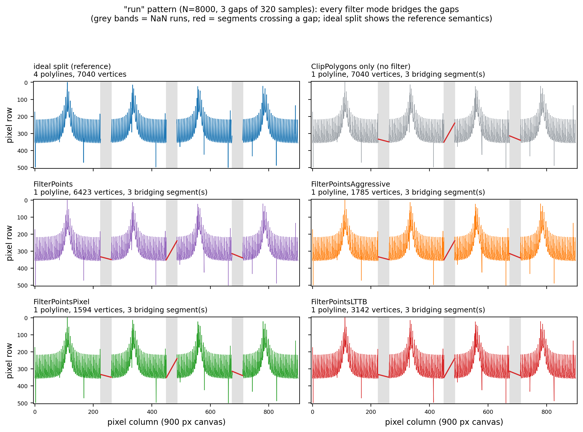
Split behavior illustrated: the ideal split reference and the actual output of the five modes; gray bands are NaN runs, red are bridging chords

4. Experiments¶

4.1 Method and reproducibility¶

The scripts and raw data of all three experiment groups are in the repository: docs/assets/algorithms/nan_experiment.py (line-by-line Python reimplementation + semantics matrix + figures), nan_mapper_check.cpp (real-library semantics harness: directed matrix, random campaign, offscreen visual scan, behavior probes), nan_bench.cpp (performance sweep, mirroring nanperf's NanDataGenerator and BenchmarkRunner decomposition), nan_results.csv (raw measurements), nan_mapper_hashes.csv (cross-validation hashes). The correspondence between the Python reimplementation and the C++ is line by line: both rounding-function quantization forms (the qwtToPoints family uses transform()'s $p_1+(v-t_1)c$ form, the Quad/Pixel/MinMax linear fast paths use the $vc + (p_1 - t_1 c)$ form), qwtFindVisibleRange's probes and two binary searches, the flush order of the Quad two-pass merge, MinMax's bucket boundary int(b*s) truncation and (value, index) first-occurrence semantics, and Qt 5.15 qRound's int32 wrap-around, all replicated from the source; the single exception is Quad's first vertex: C++ uses qwtRoundValue(xMap.transform(...)) (qwt_point_mapper.cpp line 242), while the Python side uniformly takes the linear fast path's fast() form (nan_experiment.py line 273); the two are numerically equivalent on the test signals, corroborated by the 100% hash agreement. Cross-language data always uses rational signals containing only addition, subtraction, multiplication and division (transcendental functions are not guaranteed bit-identical across libm implementations), and the random campaign shares an xorshift64* stream. Cross-validation scale: 15 directed cases × 6 paths + 250 random cases × 2 canvases (40×30 and 900×500) × 6 paths = 3090 polygon hashes, 100.00% agreement; in addition, 90 directed-case groups underwent vertex-by-vertex bit comparison (including the (899,NaN) degenerate vertex), all agreeing; that comparison was a one-off manual verification process: the committed nan_mapper_hashes.csv stores only vertex counts and quantized hashes; the C++ harness's %.17g-precision V vertex records were not committed and can only be regenerated by recompiling and rerunning the harness. The committed hashes are a pre-v7.5.0-fix run: re-running against the current library would change the matrix's all-row points case, the xyinter lttb case and others, because of the list #3/#5 fixes. The visual scan renders 960×560 images offscreen with QwtPlotRenderer: the actual render is a single curve containing NaN; the ideal reference is multiple curves split at the finite runs (same mode attribute, same pen width, same antialiasing), compared pixel by pixel in ARGB.

The semantics harness provides four subcommands: nan_mapper_check matrix prints the full vertex sequences and polygon hashes of the directed cases; random <count> <seed> runs the random campaign (data and hashes emitted in the same stream; the Python side regenerates the data with the same seed and compares); visual <outdir> runs the offscreen visual scan and writes the rendered PNGs of the run and xyinter modes to disk for manual review; probes runs the behavior probes (Steps/Sticks/Dots pixel probes, boundingRect and autoscale bounds, x-NaN/Inf spurious vertices, visible-range truncation). QwtPointMapper is exported with QWT_EXPORT in qwt_point_mapper.h, so the semantic verification of the Lines-family paths drives the mapper directly instead of guessing through pixels; Steps/Sticks/Dots live inside QwtPlotCurve's private draw functions and are instead verified at the behavior level by "probing pixels after rendering" (checking on a 1:1 canvas grab whether the neighborhood of a specific data coordinate got painted). nan_bench has four entry points: sweep A (the main NaN ratio × point count × mode sweep), B (nanperf's eight cases × mode), C (all-NaN/empty-data degenerate), and single (single-configuration tightened re-measurement).

4.2 Semantic verification results¶

The semantics matrix (the two tables of Section 3.8) gives the core correctness conclusion: the skip semantics holds on all five paths without exception, and the bridging-chord count is identically equal to the interior-gap count; Dots/Sticks are naturally correct because they are per-sample independent; under all-NaN input every path outputs an empty polygon except points, which leaves a single NaN vertex (that single vertex is a pre-v7.5.0-fix snapshot, see Section 3.2). The random campaign (NaN ratios 0–60%, x-NaN ratios 0–10%, including 4% all-NaN cases) pressed all the boundary situations (empty runs, single-point runs, alternating x/y NaN, both sides of the bucket fallback threshold) into the 100% agreement rate.

The random campaign's construction deliberately covers the boundaries of the path branches: sample counts of 3–502, so that the 40×30 canvas's bucket fallback threshold $2N_b=160$ falls inside the value range (both sides of the bucketing and Quad fallbacks get pressed), while the 900×500 canvas's threshold of 3600 is always above the sample count (MinMax's internal Quad fallback branch is taken by every case); the directed cases' N=8000 covers the true bucketing path. The y-NaN ratio is sampled uniformly over 0–60%, the x-NaN ratio over 0–10%, with an all-NaN case inserted every 25 cases. Each case runs all 6 paths under both canvases (5 user modes + lttbgen, the forced generic path); hashes are compared doubly as (vertex count, quantized vertex sequence modulo $2^{32}-5$); the vertex count is compared separately so that degenerate differences like "empty polygon vs single NaN vertex" cannot hide behind a hash coincidence. 250 cases × 2 canvases × 6 paths = 3000 random comparisons plus 90 directed comparisons, all agreeing; the directed cases additionally get a vertex-by-vertex %.17g-level comparison, 90/90 bit-identical including the (899, NaN) degenerate vertex (a one-off manual comparison: the committed hash artifacts do not contain the raw vertex sequences, so this item cannot be re-verified directly, see 4.1).

Note — Boundaries of the cross-validation

Hash agreement proves the Python reimplementation and the real library are bit-identical at the mapping-layer output; it does not cover rasterization (QPainter), clipping (QwtClipper), or layout. The NaN-related behavior of the latter three is covered independently by the offscreen rendering scan of Section 4.3 and the behavior probes of Section 4.2.

4.3 Visual correctness scan¶

Fixed signal (N=20000, containing 4 narrow +2.4 spikes and one −3.1 deep trough) × 11 NaN patterns × 5 modes; the differing-pixel fraction (%) against the ideal split rendering:

Mode	none	points	aggressive	pixel	lttb
baseline (no NaN)	0.000	0.000	0.000	0.000	0.000
isolated	1.385	1.587	0.502	1.030	2.504
run	2.004	1.116	0.229	0.785	3.627
leading	0.000	0.000	0.000	0.000	2.713
trailing	0.000	0.000	0.000	0.000	2.700
all	0.000	0.000	0.000	0.000	0.000
extremum	2.104	1.692	0.624	1.004	3.798
periodic	2.371	2.558	1.054	2.996	3.322
xynan	0.035	1.121	0.258	0.528	2.848
xyinter	0.035	1.121	0.258	0.528	2.975
spikenan	1.113	1.183	0.440	0.836	2.953

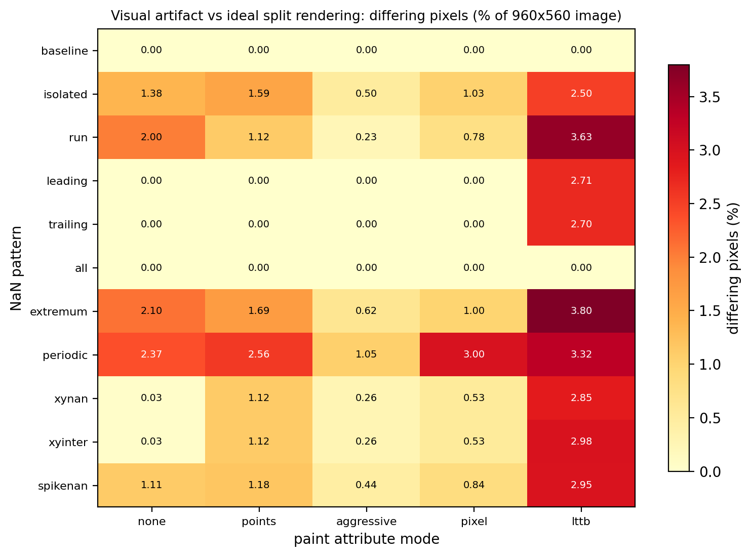
$Visual artifact heatmap: differing-pixel fraction against the ideal split rendering (data source is this section's visual scan table, not the Section 3.8 semantics matrix)$

Reading the table takes three layers. First layer: baseline and all being all-zero is the sanity check: without NaN the actual render is pixel-identical to the single-run ideal render, and with all-NaN both sides are a blank canvas. Second layer: among the patterns with interior gaps, every mode is non-zero, and the bridging chords are the bulk of the difference; aggressive is lowest (0.23%–1.05%) because the quad merge squeezes the two sides of a gap into the same column, leaving the shortest chords; none is among the highest (1.1%–2.4%) because it keeps all finite samples and the chord crosses the gap at the original slope. The third layer is LTTB's two extra terms: leading/trailing have no interior gaps and the other four modes differ by 0, yet LTTB shows 2.7%. This is not bridging but bucket-boundary reshuffling: the ideal reference spreads about 1750–1800 buckets over 18000 finite samples, while the actual curve spreads the same number of buckets over 20000 samples (NaN placeholders included) (the bucket count is twice the canvas pixel width; the canvas width was not committed separately at the time and can only be estimated from the 960-pixel-wide render minus margins), and the misaligned bucket boundaries select different extremes; the LTTB differences of the isolated/run patterns also stack the same reshuffling term (the ideal reference's short runs additionally trigger the n <= 2N_b Quad fallback). The 0.035% in the none column of xynan/xyinter also does not all come from line caps/joins at the split points: its difference bounding box (columns 454–546, rows 281–283) forms a narrow horizontal band, indicating that the bridging chord itself (the actual render spans the split point with one chord; the ideal reference has two disconnected endpoints there) accounts for about half, the rest being rasterization differences of the caps/joins, negligible in magnitude.

The spatial distribution of the differing pixels (the vis rows of nan_results.csv carry difference bounding boxes) supports the attribution above: under the run pattern, none's difference bounding box is columns 269–959, rows 247–522, spanning all three gaps and the signal region to their right, with a maximum channel deviation of 224/255, the bridging chords painted in full; aggressive's bounding box narrows to columns 270–768 under the run pattern (the third chord is absorbed by the column merge into the vertical stroke of an adjacent column), the deviation still full-scale. Under the periodic pattern (N=20000 for the visual scan, about 400 periodic gaps 5 samples wide; the CSV's ideal reference idealSegs=400, 399 interior gaps), pixel rises to 3.00%, above none's 2.37%: when empty columns are dense, the +0.25/+0.75 sub-pixel placement offsets every column's vertical stroke by half a sub-pixel from the ideal reference, and after antialiasing blending every pixel of the whole curve participates in the difference; this is a superposition of the metric and the placement rules, not a new semantic error.

The conclusion, phrased as the question "which mode draws NaN data wrong": every Lines mode draws chords that do not exist in the data, and LTTB additionally changes the shape of the finite regions through bucket reshuffling. If the business requires "gap means blank", the approach is to split on the data side (Section 6) or to enable BreakAtNan (since v7.5.0, Lines/Steps); if the requirement is only "gaps must not be glaring", aggressive's column merge squeezes the chords into vertical strokes with the smallest visual difference, at the cost of the column-merge fidelity loss discussed in Section 6.3 of Curve Downsampling. The two goals cannot be had at once; the choice belongs to the data-semantics side, not the renderer side.

4.4 Performance sweep¶

Protocol: 900×500 canvas, fixed axis ranges (X 0..N−1, Y −1.5..1.5), ImmediatePaint, offscreen platform; boundingRect is 5 cold-cache scans (cache invalidated with setSamples before each), taking the minimum; replot is 3 warm-up frames + 7 timed frames, taking the minimum and median, with extra batches appended when (median−min)/min > 30% within a batch (at most 4 rounds). Environment: i7-14700, Intel UHD 770, Qt 5.15.16, QWT Release (MSVC2019 /O2), Windows 10; absolute numbers vary with hardware, relative relations are stable.

Frame time (replot, min-of-7, ms), Middle case:

NaN%	100k none	points	aggressive	pixel	lttb	1M none	points	aggressive	pixel	lttb
0	18.77	17.62	5.03	9.85	6.81	173.67	159.48	25.16	81.66	26.25
1	19.73	18.04	6.94	9.85	5.28	159.25	145.02	22.62	75.59	24.69
5	18.65	17.42	5.34	9.87	5.25	162.95	145.54	22.93	75.50	23.04
10	17.21	14.72	4.84	8.89	4.81	147.95	129.30	20.82	69.09	22.76
25	15.53	13.36	4.15	8.30	4.29	124.22	113.65	20.29	59.24	18.13
50	9.81	9.44	3.38	6.96	3.42	86.50	83.65	15.31	42.54	13.06

boundingRect cold scan (min-of-5, ms, min–max interval over the five modes):

NaN%	100k	1M
0	2.0–2.3	19.6–21.7
10	1.8–2.7	16.6–19.6
50	1.3–1.4	11.5–12.8
100 (all NaN, sweep C)	0.51–0.56	not measured
empty data (sweep C)	0.0000	not measured

The boundingRect measurement convention needs a separate note: it measures a cold-cache scan: setSamples is called before each timing to invalidate QwtPlotSeriesItem's cached rectangle, so the numbers represent the one-off cost "right after the data updates", not a per-frame cost. The table gives the min–max interval over the five modes rather than a single value because this scan is independent of the paint attribute (the same qwtBoundingRectT code), and the differences between modes are purely cache-state noise; the interval width is about 2 ms at 1M points, exactly the magnitude of memory-system noise. nanperf reports about 8.6 ms for 100k points in the GUI scenario, four times the offscreen ~2 ms measured here; the difference comes from panel layout and the event loop's cache state. The two agree on the direction of response to the NaN ratio (nanperf drops to 3.2 ms at 99% NaN; this article drops to 1.3–1.4 ms at 50% and 0.5 ms at all-NaN).

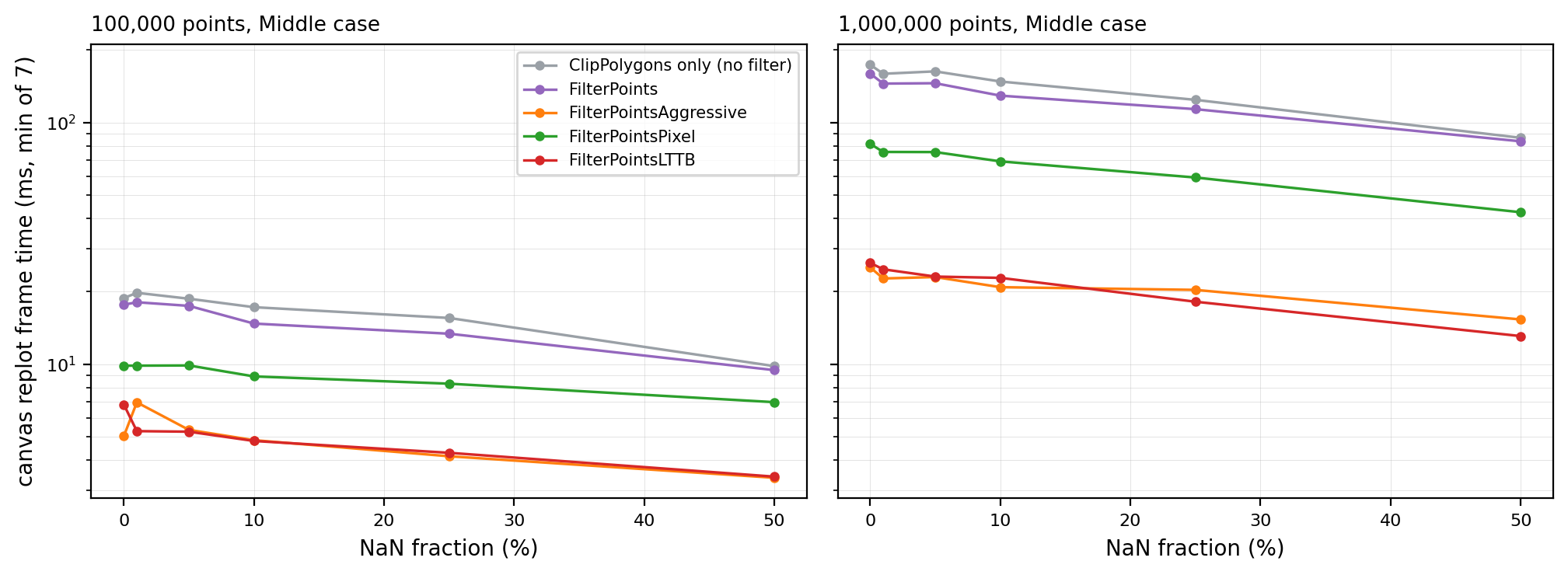
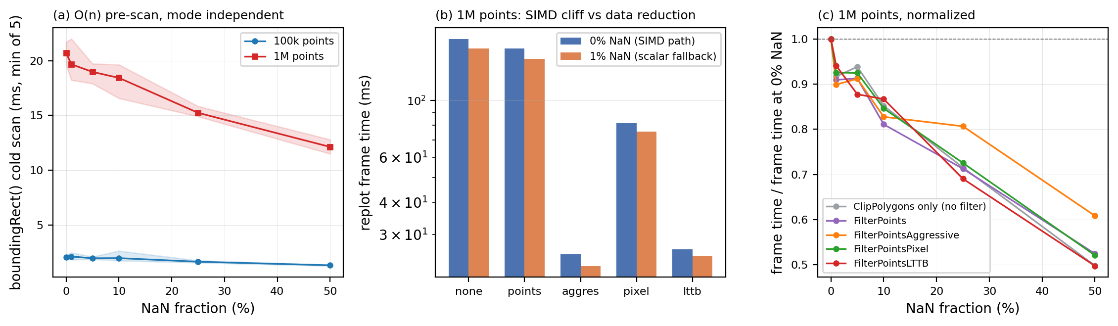
NaN ratio–frame time curve families (grouped by mode, log axis)

Cost breakdown: boundingRect pre-scan, SIMD cliff, and data reduction

Three readings. First, frame time decreases overall with the NaN ratio (individual 1%/5% cells rebound within measurement noise, see 1M none 1%→5% in the table above); the normalized curves of the modes are close but do not fully coincide (panel (c) of the cost-breakdown figure fig_nan_breakdown above: at 50%, none/points/pixel/lttb drop to about 0.50, aggressive slightly higher at about 0.61). NaN's net effect is data reduction: fewer finite samples to transform, rasterize, and clip. The 1M-point no-filter mode drops from 173.7 ms to 86.5 ms (0→50%), LTTB from 26.3 ms to 13.1 ms. Second, boundingRect's O(n) scan likewise eats the data reduction: 1M points drop from about 21 ms to about 12 ms, because skipped samples do not participate in the min/max extension; at all-NaN, 100k points take only 0.5 ms (just the isfinite decision), and empty data 0. Third, the SIMD cliff is invisible at frame level: by nanperf's analyze() convention, the 0%→1% ratio for 100k-point LTTB is 0.776 against a mean ratio of 1.064 for the other modes, delta = −0.29 (LTTB benefits more from data reduction); at 1M points the ratios are 0.941 against 0.915, delta = +0.03 (marginal). At 100k points there is even a counterintuitive cell: LTTB at 0% (SIMD path) is 1.5 ms slower than at 1% (scalar path), because with buckets of about 55 samples the fixed overhead of one qwtSimdArgMinMax call per bucket (vector loads and horizontal reduction) exceeds the parallelism gain (Section 5.4 of Curve Downsampling makes the same argument for this threshold), and at 0% it is stacked with the full $O(n)$ read that the pre-scan cannot short-circuit. Frame time is rasterization-dominated (mapping is only a small part of the 173.7 ms of 1M no-filter), and the SIMD/scalar difference of the bucket reduction is buried inside it; observing the pure reduction cost requires a microbenchmark, which this report does not attempt.

Distribution-case sweep (sweep B, 100k points, 10% NaN, replot min, ms):

Case	none	points	aggressive	pixel	lttb
baseline	18.20	17.41	5.17	9.59	5.26
leading	15.66	14.53	4.27	9.03	4.73
leadtrail	16.25	15.55	4.72	8.95	4.42
middle	16.59	15.67	4.70	9.09	4.82
trailing	16.99	15.48	4.74	9.42	4.60
xynan	16.20	14.87	3.57	8.60	4.61
xyinter	15.70	15.87	3.60	9.11	5.13
allnan	1.58	1.79	1.44	1.31	0.69

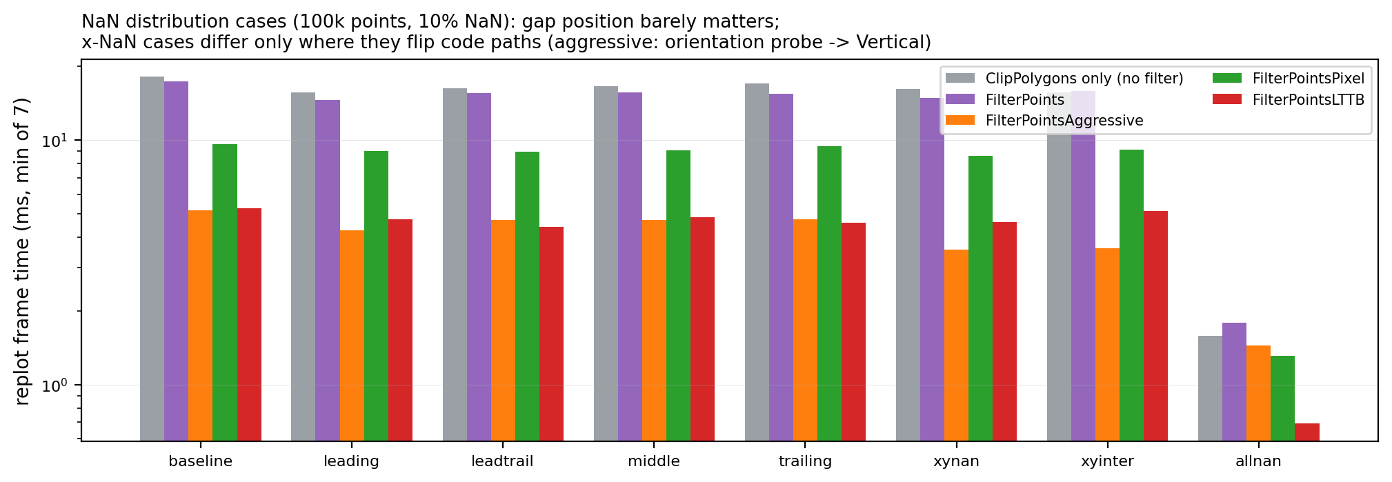
Distribution-case frame times: gap position has little effect; x-NaN makes a difference only where it flips a code path

Gap position (leading/middle/trailing/leadtrail) affects frame time within ±10%, consistent with nanperf's "position does not affect performance" conclusion; the differences of the two x-NaN cases come from Section 3.3's orientation-probe flip (aggressive) and Section 3.5's spurious-vertex extra rasterization (xyinter's lttb is about 6% slower than middle). Degenerate data (sweep C): all-NaN frame time 0.63–1.72 ms, empty data 0.54–0.56 ms, the noise floor of "drawing axes only". Combined with Section 3.1's invalid bounding rect and the 0–1000 axis fallback, the complete behavior of an all-NaN curve is blank canvas, default axes, and no crash.

Converting to frame rate (fps = 1000/frame-time minimum) aligns with nanperf's tables: at 100k points and 10% NaN, lttb is about 208 fps and none about 58 fps; at 1M points and 0% NaN, lttb about 38 fps and none about 5.8 fps; at 1M points and 50% NaN, lttb about 77 fps. The all-NaN 100k curve reaches about 1576 fps with lttb; by then the frame time is entirely the noise floor of the axes and canvas clearing, independent of the data volume. The absolute values nanperf reports on the GUI thread with grid and panel layout (100k, no NaN, lttb about 12.4 ms) are higher than the offscreen single-curve values here (5.26 ms); the difference comes from scene composition, not pipeline semantics. The two agree on the ordering among modes and on the overall trend of frame time decreasing with the NaN ratio.

4.5 Measurement integrity notes¶

Other benchmark tasks ran in parallel on the machine during timing. The first round of sweep A had 2 configurations with within-batch spread above 30% (1M pixel 0%, 1M none 10%); extra batches were appended and re-measured per protocol. A subsequent full re-run (adopted as this article's main data) has spread < 25% on all 110 rows and mutually corroborates with the single-configuration tightened re-measurements (sweep=S rows): pixel 1M 0% has 3 min-of measurements in total, 76.3/81.7/85.2 ms (two re-measurements plus the main data; interval 76.3–85.2); none 1M 10% has only 1 re-measurement batch, 2 measurements together with the main data, 138.9/147.9 ms. The only non-converged cell is lttb 1M 0%: the main session's min-of is 26.3 ms, and the two independent re-measurements leave two readings in the sweep=S rows of nan_results.csv, 31.8/34.9 ms and 35.4/37.3 ms (both column conventions are listed side by side, not mixed with the article-wide min-of main convention); the batch-level raw data was not committed, so the within-batch spread cannot be re-verified; all that can be given is (median−min)/min = 6.8% and 11.5% for the two re-measurement rows. The two session clusters are each internally relatively stable and clearly separated from each other, attributed to clock state under concurrent load; the min-of protocol keeps the quiet-session value, nan_results.csv retains the re-measurement records as sweep=S rows, and readers may take the conservative value themselves. The relative relations (the ordering among modes, the overall trend of frame time decreasing with the NaN ratio) are consistent across all sessions.

5. Discussion: failure modes¶

Update record (v7.5.0)

This article is a point-in-time snapshot from 2026-10; the conclusions and measured numbers in the body stay as they were. Three items of the list below have since been fixed, and one has gained a library-level outlet:

Naming first: since v7.5.0 FilterPointsLTTB maps to the true LTTB (QwtPointMapper::LTTBReduce, qwtLttbReduce()) and the MinMax bucket algorithm analyzed in this article moved to the new attribute FilterPointsMinMaxLTTB (MinMaxReduce). The "LTTB raw-pointer path" of item 3 below means the MinMax bucket path (FilterPointsLTTB was that implementation up to v7.4.2), as do the lttb modes of Sections 3.5/3.8 and the Section 4 performance data. The raw-pointer branch of the true LTTB (qwtLttbReduce's mapSample, lines 915–922) still decides sample validity with std::isnan(y) alone, so non-finite x and ±Inf y enter its selection, the same class of predicate as #3/#4 that was fixed on the MinMax side persists on the new default path, so the cleaning advice of Sections 6.2/6.4 still applies to the default mode.

#3 (LTTB x-NaN phantom vertex) and #4 (Inf passing the pre-scan) are fixed: the pre-scan predicate is now !isfinite(y) (rejecting Inf); non-finite x values are caught by a per-bucket post-check in the SIMD path (only when a raw x pointer exists, hasRawX), and affected buckets are recomputed with the scalar loop (reduceBucketScalar(b)); the scalar bucket loop skips samples with a non-finite x or y, and the raw-pointer path now matches the generic path's semantics and no longer emits (0, y) phantom vertices or INT_MIN garbage coordinates (regression tests: tests/nan_curve_test, lttb_xNan_noPhantomVertex/lttb_inf_noGarbageCoordinates). Note: scanning x in the pre-scan as well was measured to cost +11% frame time on 1M clean lttb points (double array memory traffic), hence the per-bucket post-check design.

#5 (FilterPoints single vertex on all-NaN) is fixed: qwtToPolylineFiltered gained an all-NaN early exit (lines 1245–1248); all-NaN input returns an empty polygon, restoring the "empty polygon = no data" convention (regression test filterPoints_allNan_emptyPolygon).

#1/#2 (bridging semantics) gained a library-level outlet: the QwtPlotCurve::BreakAtNan curve attribute (qwt_plot_curve.h line 177, off by default) switches Lines/Steps to split semantics — every finite run is rendered, filled and smoothed independently (drawLines lines 682–697, drawSteps lines 947–962, the drawDots fill branch lines 807–822), gaps stay blank; data-side splitting (Section 6.1) remains available. The finite-run index ranges are cached by finiteSampleRuns() (qwt_plot_curve.cpp lines 119–158) and invalidated on data changes.

#6/#7/#8 unchanged: #6 is inherent to bucketed downsampling, #7 has no visual loss, and the use-guide lag of #8 has been synced with the fixes (both EN and ZH).

#	Failure	Trigger condition	Measured evidence	Impact
1	Bridging chord: a NaN run is spanned by a segment that does not exist in the data	any interior NaN run + any Lines mode/Steps	bridged equals intGaps throughout the semantics matrix; visual difference 0.23%–3.80%	the gap is "welded shut" and misread as a continuous signal
2	Steps' bridging geometry is worse: the vertical jump moves forward to the gap's left edge	Steps + interior gap	probes tread=1, riser=1, pre_level=0	the step changes level before the gap
3	LTTB raw-pointer path's x-NaN spurious vertex: the pre-scan and the scalar bucket loop check y only; when an x-NaN sample wins a bucket extreme, screen x = `qRound(NaN)` = 0 (fixed in v7.5.0)	x contains NaN and that sample is a bucket extremum	`xnan_lttb_fakeLeft=1`, polygon contains (0,21); xyinter vertices 3567 vs generic path 3215 (both pre-fix snapshots)	a spurious spike appears at the canvas's left edge
4	Inf passes through the `isnan`-only pre-scan into the SIMD path (fixed in v7.5.0)	y contains ±Inf	`inf` case: lttb garbage coordinates 1; `qRound(+Inf)=INT_MIN`, `qRound(-Inf)=0`	spurious lines at the top/bottom edges or flying points
5	FilterPoints outputs a single-vertex (x, NaN) polygon on all-NaN (fixed in v7.5.0)	all-NaN + FilterPoints	matrix all row, points: 1 vertex, 1 garbage	the polygon is non-empty; downstream assuming "empty = no data" misjudges
6	LTTB bucket reshuffling: NaN occupies the bucket budget; the shape of the finite regions changes with gap position	any NaN + LTTB	leading/trailing visual difference 2.7% (nonzero with no bridging at all)	not equivalent to "rendering run by run"; export/comparison scenarios need care
7	The visible-range binary search over-scans for isolated x-NaN that dodge the probes	sparse x-NaN + zoomed axis	probes: coverage is still the full canvas width, no truncation	extra computation only, no visual loss
8	Documentation lag: the use guide says Sticks/Steps/MinimizeMemory do not check NaN	—	the current source has `isSampleNanOrInf` checks at all four places (commit 17d0d13)	documentation-only issue; the semantics remains skip

Items 1 and 2 of the list are semantic choices, not defects: the skip semantics is QWT7's improvement direction relative to Qwt 6 (in the 6 era NaN produced wild pixel coordinates), and split semantics was never promised. Items 3 and 4 genuinely deserved reporting at the time: they made paths that "checked NaN" still emit geometrically nonexistent vertices, and both fixes were low-cost (item 3: add one isfinite check on x in each of the pre-scan and the scalar bucket loop, or switch to qwt_is_nan_or_inf on the (x,y) pair; item 4: replace the pre-scan predicate isnan with !isfinite). Both landed in v7.5.0 along those lines: item 4 by simply swapping the predicate, item 3 via the per-bucket x post-check for performance reasons. Residual issue: the true LTTB introduced in v7.5.0 (now the default FilterPointsLTTB) still checks isnan(y) only in its raw-pointer branch, so the same class of samples as #3/#4 still enter its selection (see the first update-record item); until that path is fixed, data whose x contains NaN or ±Inf should be cleaned before entering any LTTB bucket algorithm. Item 5 is harmless but breaks the downstream convention "empty polygon = no data" and deserves a note in the API documentation (v7.5.0 fixed it with the empty-polygon early exit). Item 6 is an inherent property of bucketed downsampling (bucket boundaries depend on sample counts): split rendering and whole-sequence rendering are mathematically nonequivalent, and documentation is the only remedy. Item 7 is confirmed by probes to have no visual loss; recording it suffices. Item 8 reminds readers that the lagging conclusions between this article and the use guide are more than one: style-coverage content appears in two places in the guide (the drawing-style coverage table and its warning, and the "Choosing a Drawing Style" paragraph of "Best Practices"), and the autoscale code snippet also disagrees with the current source; the current source is authoritative in all cases (this revision has corrected the guide in sync).

Comparison with the nanperf example: nanperf's 8-case matrix (Baseline/Leading/LeadingTrailing/Middle/Trailing/XyNan/XyInterleavedNan/AllNan) is mirrored verbatim by sweep B, and its BenchmarkRunner's three-part boundingRect/replot/fps decomposition is inherited by nan_bench.cpp; the SIMD-cliff delta convention is applied here, recomputing the same formula on nan_results.csv (Section 4.4, third reading; nan_bench.cpp contains no analyze code); this article extends it with six more semantic patterns (isolated/periodic/extremum/xonly/inf/spikenan), the per-pixel visual scan, and the 1M-point scale. The deltas recorded in nanperf's documentation (−0.19 at 1%, +0.03 at 99%) and this article's (−0.29 at 100k, +0.03 at 1M) have the same sign and magnitude; the conclusion "the SIMD cliff is negligible, data reduction dominates" is mutually corroborated by two independent implementations. The difference is that this article explains the mechanism behind "negligible" in more detail: the cliff is masked not because the scalar fallback is cheap, but because the rasterization-dominant term of the frame time and the pre-scan short-circuit effect cancel it in the same direction.

The skip semantics also buys something, and the discussion should be symmetric. A single QPolygonF keeps the downstream pipeline simple: ClipPolygons's one clip pass, render smoothing (Gaussian/Savitzky-Golay, see the curve smoothing article)'s continuous neighborhood windows, and the Fitted attribute's curve fitting all assume the input is one connected polyline; split semantics would require every one of these stages to be changed to "process run by run + no filtering across runs", otherwise the smoothing kernel would cross the gap and pollute the two sides' signals with each other, the bridging chord at least keeps the smoothing window's behavior identical to the NaN-free case (at the cost of losing half a window's fidelity on each side of the gap). On performance, the skip semantics' mapping cost is independent of NaN position (sweep B's ±10%), and in implementation the five paths need only one continue, with no segment table or inter-segment state to maintain. QWT7 therefore trades gap visibility for pipeline uniformity, a trade that pays off for monitoring-wall-type scenarios and does not for scientific-publication-type scenarios; the criterion is whether readers will read the bridging chord as data.

Warning — A gap is not a blank

In QWT7, a polyline containing NaN does not leave a blank at the gap (unless BreakAtNan is enabled, which covers Lines/Steps only). Any downstream that reads NaN as "disconnected" (reports, alarm screenshots, paper figures) must split explicitly on the data side, enable BreakAtNan, or accept the bridging chord and explain it in the caption.

6. Code practice¶

6.1 Data side: the explicit way to make a gap a gap¶

Since v7.5.0 the BreakAtNan curve attribute can also split Lines/Steps into runs on the rendering side (see the Section 5 update record); this section gives the data-side approach, which needs no attribute and applies to every paint mode and every pipeline stage. For the ideal split semantics, cut the sequence into multiple runs at NaN before feeding it to the curve, one curve per run, exactly how the visual scan's ideal reference is constructed:

#include <qwt_plot.h>
#include <qwt_plot_curve.h>
#include <cmath>

// Split a NaN-marked series into one curve per finite run: gap semantics
// independent of the BreakAtNan attribute and of the paint mode.
void attachSplit(QwtPlot* plot, const QVector<double>& x, const QVector<double>& y)
{
    int start = -1;
    for (int i = 0; i <= x.size(); ++i) {
        const bool finite = (i < x.size()) && std::isfinite(x[i]) && std::isfinite(y[i]);
        if (finite && start < 0) {
            start = i;
        } else if (!finite && start >= 0) {
            QwtPlotCurve* c = new QwtPlotCurve();
            c->setSamples(x.mid(start, i - start), y.mid(start, i - start));
            c->attach(plot);          // each run is downsampled and clipped independently
            start = -1;
        }
    }
}

The cost is the item-management overhead as the number of runs grows, plus the independent downsampling budget per run (short runs fall back to the quad merge); below about a hundred runs no perceptible difference is expected (this article made no quantitative measurement of multi-item overhead). If the business can accept bridging (e.g. gaps narrower than one pixel column), a single curve + skip semantics saves memory.

6.2 Mode selection and data hygiene¶

Scenario	Recommendation
gaps must display as blank	split on the data side (6.1) or enable the `BreakAtNan` curve attribute (Lines/Steps, since v7.5.0); any mode
bridging accepted, frame rate pursued	default `FilterPointsLTTB`; the gain is larger at high NaN ratios (13.1 ms at 1M points, 50%)
levels on the two sides of the gap are close, chords unobtrusive	`FilterPointsAggressive` (lowest visual difference, 0.23%–1.05%)
x coordinates may contain NaN	clean x first: the MinMax-bucket raw-pointer path used to emit a spurious vertex for x-NaN (list #3, fixed in v7.5.0); the true LTTB (the default `FilterPointsLTTB`) still checks `isnan(y)` only in its raw-pointer branch, so non-finite x enters the selection; cleaning is the safest option
data may contain ±Inf	clean with `qwtRemoveNanOrInf`: the MinMax pre-scan rejects ±Inf since v7.5.0 (list #4 fixed), the true-LTTB raw-pointer branch still lets ±Inf through; cleaning is the cheapest defense
all-NaN / empty sequence	no special handling needed: invalid bounding rect, axes fall back to 0–1000, blank canvas, no crash; but the automatic axes are meaningless; an explicit `setAxisScale` is recommended
Sticks / Dots	skipping is the correct semantics, use directly; Steps has bridging (list #2)

The "best practices" section of the use guide NaN Data Handling gives the tutorial view of marking missing samples with qQNaN() and of boundingRect skipping them automatically; Sections 2 and 3 of this article explain the comparison semantics behind those behaviors, and the Section 5 list supplements their boundaries. The two articles agree completely on "skip"; the guide's formerly lagging content involved the two style-coverage places (the coverage table and its warning, the best-practices paragraph) and the autoscale code snippet (list #8, corrected in sync in this revision); the current source is authoritative in all cases.

6.3 Performance-side practice¶

boundingRect's cold-scan cost (about 12–22 ms at 1M points) occurs once per data change (QwtPlotSeriesItem caching), so scrolling-window scenarios need not worry; but if the series object is rebuilt every frame (a common pattern for streaming data), this $O(n)$ enters the per-frame budget. There, the higher the NaN ratio, the cheaper it gets (pre-scan short-circuit + skipped extension). When it must be recomputed every frame and the data has no NaN, keeping the default suffices; when the data contains NaN and LTTB is used, remember that the scalar and SIMD bucket loops are almost the same price at frame level (Section 4.4, third reading); there is no need to clean NaN just to "keep SIMD".

6.4 Data hygiene before entering the LTTB raw-pointer path¶

Against list items 3 and 4, the cheapest defense is to clean x and y jointly by (x,y) pair before setSamples. The core module's qwtRemoveNanOrInfCopy (src/core/qwt_math.h) is a template that filters NaN/Inf elements from a single container: calling it separately on the x and y containers breaks index alignment the moment the two sides drop different numbers of elements, the most common wrong pattern. The correct approach is a joint filter loop with a both-coordinate predicate:

#include <qwt_math.h>
#include <qwt_plot_curve.h>

// Sanitize before feeding the LTTB raw-pointer path: drop every sample whose
// x OR y is NaN/Inf, filtered jointly over (x, y) pairs so the two vectors
// stay index-aligned. This kills the phantom-vertex and Inf hazards (items
// 3, 4 of the failure list). Gaps are still bridged afterwards - split first
// (6.1) if gap semantics are required.
QVector<double> xs, ys;
xs.reserve(xRaw.size());
ys.reserve(yRaw.size());
for (int i = 0; i < xRaw.size(); ++i) {
    if (!qwt_is_nan_or_inf(xRaw[i]) && !qwt_is_nan_or_inf(yRaw[i])) {
        xs.append(xRaw[i]);
        ys.append(yRaw[i]);
    }
}
curve->setSamples(xs, ys);

Equivalently, organize the data as QVector<QPointF> and call qwtRemoveNanOrInfCopy directly: its predicate lands on the both-coordinate overload qwt_is_nan_or_inf(const QPointF&), filtering by (x,y) pair naturally, which is exactly why that overload exists. The semantic boundary of this cleaning also matters: it removes "samples whose x or y is NaN/Inf"; for y-only gaps this is precisely the opposite of split semantics (the two sides are still bridged after removal), so it solves the spurious-vertex and Inf problems, not the gap-semantics problem. If the data source guarantees monotone finite x (as the vast majority of time-series acquisition does), confirming that y has no Inf suffices to avoid item 4, and item 3 cannot trigger.

7. Summary¶

QWT7 has governed NaN from a "crash source" (Qwt 6's polluted bounding rects and wild pixels) into a "skipped sample": all five mapping paths, the four curve styles, and the whole bounding-rect-and-autoscale chain carry explicit isfinite checks. The price of this governance is a semantic choice: skip-not-split. The semantics matrix, the 3090 cross-validations and the per-pixel visual scan quantify the consequences down to the pixel: every interior gap produces exactly one bridging chord in all Lines modes, the difference against the ideal split rendering lies between 0.23% and 3.80% of pixels, and LTTB stacks a bucket-reshuffling term on top. The performance side is far milder: NaN's net effect is data reduction, both frame time and pre-scan cost decrease with the NaN ratio, and the SIMD cliff is masked at frame level (delta −0.29 / +0.03). The boundaries remain clear: readers who need "gap means blank" can enable BreakAtNan (Lines/Steps, since v7.5.0) or split on the data side themselves; data whose x contains NaN or Inf must be cleaned before entering the raw-pointer path of any bucket algorithm (including the true LTTB). Whether the skip semantics is QWT's long-term answer (v7.5.0 has given a split switch at the curve-attribute layer, BreakAtNan, while the mapper layer still has no split flag) is a design question; the measurements here only cover the status quo and its cost.

Semantic judgment: QWT7's NaN handling is "crash-prevention governance", not "gap-semantics design"; using it as matplotlib-style splitting produces systematic misreading, and bridging chords are unacceptable in scenarios with wide gaps and large level differences.
Correctness boundary: the skip semantics happens to be correct on Dots/Sticks, happens to be wrong on Lines/Steps, and adds one more layer of bucket-reshuffling bias on LTTB; the same data changes semantics as soon as the style changes, and the interface layer makes no uniform promise.
Performance boundary: NaN introduces no superlinear cost, the pre-scan and the bucket loop are both $O(n)$ with small constants; the frame-time gain comes from data reduction, with speedups of 1.6–2.0× across modes at 1M points and 50% NaN (aggressive 1.64, points 1.91, pixel 1.92, lttb 2.01, none 2.01).
Measurement boundary: frame-level measurements cannot isolate the pure difference between the SIMD and scalar bucket reductions (rasterization dominates); this report gives frame-level facts and mechanism hypotheses only; lttb 1M/0% has a session-level double cluster of 26 vs 32–37 ms (re-measurement readings 31.8/34.9, 35.4/37.3), taken per the min-of protocol with the re-measurement rows retained.
Maintenance boundary: list items 3 and 4 (x-NaN spurious vertex, Inf passing through the pre-scan) are fixed in v7.5.0; but the true LTTB (now the default FilterPointsLTTB) keeps the same y-only isnan test in its raw-pointer branch (see the Section 5 update record), so x and ±Inf must be cleaned before it; item 6 (bucket reshuffling) is a mathematical inevitability of bucketed downsampling and deserves documentation.

8. References¶

IEEE Computer Society. IEEE Standard for Floating-Point Arithmetic (IEEE 754-2019): ordered/unordered comparison predicates and NaN propagation rules.
QWT7 sources: src/plot/qwt_point_mapper.cpp (qwtToPolylineFiltered 1222–1268, qwtMapPointsQuad 218–345, qwtFindVisibleRange 349–418, qwtPixelColumnReduce 422–535, qwtMinMaxBucketReduce 625–863, qwtLttbReduce 877–1068, qwtToPoints 1135–1194, toPolygonF 1493–1530).
QWT7 sources: src/plot/qwt_plot_curve.cpp (drawLines 583–698, drawSticks 710–756, drawDots 768–858, drawSteps 871–963), src/core/qwt_series_data.cpp (qwtBoundingRectT 217–261), src/core/qwt_simd_argminmax_avx2.cpp (the AVX2 kernel and the _CMP_LT_OQ ordered predicate), src/core/qwt_simd_argminmax.cpp (the SSE4.2/scalar paths and the runtime dispatch).
QWT7 example: examples/2D/nanperf (NanDataGenerator's eight-case matrix, FilterModes.h's five modes, BenchmarkRunner's boundingRect/replot/fps decomposition and SIMD-cliff delta analysis).
This article's companion experiments: docs/assets/algorithms/nan_experiment.py, nan_mapper_check.cpp, nan_bench.cpp, nan_results.csv, nan_mapper_hashes.csv.
Commit 17d0d13 "fix(nan): add NaN skip to 4 missing paths in QwtPlotCurve": where the four skip checks for Sticks/Steps/Dots-MinimizeMemory were introduced.

Companion reading: Downsampling Curves for the Screen: LTTB Theory and the QWT7 MinMax Bucket explains where the three paths and the bucket budget come from; NaN Data Handling (use guide) gives the tutorial view of configuration and data preparation.