Color Science of the Scientific Colormaps: Perceptual Uniformity of the 22 QwtColorMapPreset Palettes and a Scenario-Based Selection Guide

Abstract — A colormap is a mapping from data values to colors, and its quality decides whether readers "see structure that is not in the data": a ramp with non-monotonic lightness draws false contours over a smooth field, a ramp with uneven steps exaggerates certain value ranges, and to a red-green colorblind observer the whole ramp may collapse into two or three colors. QWT7's QwtColorMapPreset (src/core/qwt_colormap_preset.h/.cpp) provides 22 presets. The evaluation reproduces the 256-level LUT construction of colorTable256() bit-for-bit as implemented in src/core/qwt_colormap.cpp, with a self-implemented full chain of sRGB → linear RGB → XYZ(D65) → CIELAB, the complete CIEDE2000 formula (self-tested against the published data of Sharma et al. 2005, maximum error 4.17e-5 over 22 pairs) and the Machado et al. 2009 color-vision-deficiency simulation matrices, and evaluates the presets quantitatively along four dimensions: lightness monotonicity, uniformity of adjacent-level steps, distinguishability under color-vision deficiency, and grayscale-print safety. A scenario-based selection guide across data type × observer × output medium follows, together with several engineering facts about the preset data itself (in the first release the color stops of inferno were taken from the t∈[0,0.7] segment of the reference curve, and turbo approximately so, yet placed at positions [0,0.875]; the intermediate stops of viridis/magma/cividis deviated from the matplotlib colors at the same positions by up to ΔE00 11.4–17.2; since v7.5.1 these five presets have been resampled from the official matplotlib tables).

Abstract — Core conclusions

• Classified by objective criteria, the 22 presets are 16 sequential, 4 diverging and 2 cyclic; the color stop data of rainbow and hsv are completely identical in the source (qwt_colormap_preset.cpp:116-128)
• Lightness monotonicity: 18 of the 22 presets have zero violating steps along the dominant direction (10 of them with a cumulative regression of exactly 0); jet has 77 violating steps, a cumulative regression of 71.76 L* and a maximum regression of 70.67 L* (L* climbs to 97.14 at t≈0.625 and then falls back to 26.47; every lightness value inside (26.47, 97.14) appears once on the ascending branch and once on the descending branch, up to one quantization step of error), and turbo registers 65.52/65.52; both are graded non-uniform
• Step uniformity (coefficient of variation CV of the adjacent-level ΔE00): gray is best at 0.228, followed by rdylgn 0.326 and rdylbu 0.354; inferno/magma sit at 0.364/0.361 (0.587/0.582 before the v7.5.1 fix, which resampled the stops from the official matplotlib tables over the full [0,1] domain), close to matplotlib's own 0.332/0.348 with the remainder coming from the 9-stop linear interpolation
• Color-vision deficiency (Machado severity 1.0; the minimum ΔE00 between levels 32 apart serves as the distinguishability lower bound): coolwarm 9.96–10.30 and rdylbu 8.87–13.24 stay robust under all three deficiencies; rainbow/hsv fall to only 0.130 under deutan (t=0.620 and t=0.745 the same color), and rdylgn to 0.182; the two sides of the center are entirely indistinguishable to red-green colorblind observers
• Grayscale printing: the two ends of coolwarm differ by only ΔL* 0.36, so all sign information is lost after conversion to grayscale; the ends of rdylbu/rdylgn/spectral differ by ΔL* 4.62–5.93 and remain distinguishable; the L* of jet/turbo/cool is non-monotonic, so grayscaling them necessarily produces false contours

---

1. Introduction: why colormaps need color science

1.1 Three failure modes, formalized

Treat a colormap as the function \(c: [0,1] \to [0,255]^3\) (after discretization through a 256-level LUT, \(c_i,\ i=0..255\)), passed on to the human eye through the display's electro-optical transfer. A reader's judgment of the data rests almost entirely on three perceptual quantities: lightness (CIELAB \(L^*\)), color difference (\(\Delta E_{00}\)) and hue direction. The corresponding failure modes can be written as three measurable propositions:

1. False lightness boundaries: \(\exists\, t_1 < t_2\) such that \(L^*(t_1) > L^*(t_2) + \tau\). The human eye is extremely sensitive to lightness steps (edge-enhancement mechanisms), and a ramp whose \(L^*\) first rises then falls paints a bright band over a smooth data field that does not exist. The cyan-to-yellow transition of MATLAB's jet is the textbook case; our measurement puts its cumulative regression at 71.76 L*.
2. Uneven steps: fluctuation of the adjacent-level color difference \(\Delta E_{00}(c_i, c_{i+1})\) visually exaggerates some value ranges and compresses others. The coefficient of variation \(\mathrm{CV} = \sigma/\mu\) measures this unevenness; the larger the \(\mathrm{CV}\), the less "one color step apart" can be trusted as a statement about the underlying data difference.
3. Loss of injectivity: after color-vision-deficiency simulation or grayscaling, \(\exists\, |t_1 - t_2| \ge \delta\) such that \(\Delta E_{00}(c'(t_1), c'(t_2)) \approx 0\): two data values far apart look identical. Red-green colorblindness (protan/deutan, together roughly 8% of males) collapses the red-green opponent axis and is the main source of this failure mode.

These three propositions map one-to-one onto the three metrics of Section 2: monotonicity statistics of the \(L^*(t)\) profile, the distribution of adjacent-level \(\Delta E_{00}\), and the minimum far-apart color difference under simulated vision.

1.2 Why the evaluation runs at the LUT level

QWT has two rendering paths: the continuous path calls QwtColorMap::rgb(vMin, vMax, value) per pixel; the indexed path calls colorIndex() to look up the 256-level table generated by colorTable256() (QImage::Format_Indexed8, see Section 3.3). The evaluation uses the 256-level LUT throughout, for two reasons: it is the discretization actually used by Indexed-format rendering (which requires an explicit setFormat(QwtColorMap::Indexed); the preset factory defaults to RGB format) and by color bar ticks, and it is the limit of what an 8-bit indexed output can express; conclusions for the continuous path follow by interpolation from the LUT conclusions, but not vice versa (the continuous path may be smoother than the LUT, never worse). The LUT sampling grid reproduces colorTable256() exactly: \(\text{pos}_i = i/256\); it never reaches 1.0, so viridis has LUT[255] = (251,231,37) rather than the last color stop (253,231,37). This off-by-one is by design (qwt_colormap.cpp:282-284), and a reminder that the choice of evaluation grid itself affects the last digits.

1.3 Division of labor with the use guide

docs/use-guide/general/colormap.md covers how to use the 22 presets, the example UI and the pitfall checklist; the metrics and the evidence behind those conclusions are in this report: every "recommended" or "not recommended" corresponds to a number in one of the tables here. The two are best read as companions.

2. Color spaces and metrics

2.1 sRGB → linear RGB → XYZ → CIELAB

The 8-bit sRGB components are first normalized to \([0,1]\) and de-gamma'd through the electro-optical transfer function of IEC 61966-2-1:

\[ c_{\text{lin}} = \begin{cases} c / 12.92, & c \le 0.04045 \\ \left( \dfrac{c + 0.055}{1.055} \right)^{2.4}, & c > 0.04045 \end{cases} \]

Linear RGB is converted to CIE XYZ (D65 white point) through the standard sRGB matrix:

\[ \begin{pmatrix} X \\ Y \\ Z \end{pmatrix} = \begin{pmatrix} 0.4124564 & 0.3575761 & 0.1804375 \\ 0.2126729 & 0.7151522 & 0.0721750 \\ 0.0193339 & 0.1191920 & 0.9503041 \end{pmatrix} \begin{pmatrix} R_{\text{lin}} \\ G_{\text{lin}} \\ B_{\text{lin}} \end{pmatrix} \]

then to CIELAB as defined in CIE 15:2004, with the D65 white point \((X_n, Y_n, Z_n) = (0.95047,\ 1.00000,\ 1.08883)\):

\[ f(t) = \begin{cases} t^{1/3}, & t > \varepsilon \\ \dfrac{\kappa t + 16}{116}, & t \le \varepsilon \end{cases}, \qquad \varepsilon = \frac{216}{24389},\quad \kappa = \frac{24389}{27} \]

\[ L^* = 116\, f(Y/Y_n) - 16, \qquad a^* = 500\left( f(X/X_n) - f(Y/Y_n) \right), \qquad b^* = 200\left( f(Y/Y_n) - f(Z/Z_n) \right) \]

\(L^*\) is perceptual lightness: the gray levels on paper in grayscale printing are determined by it, so Section 4.6 treats \(L^*(t)\) directly as the grayscale profile. Implementation self-test (output of script section 1): \((255,0,0) \to (53.2408, 80.0925, 67.2032)\), within 9.4e-5 of the literature value; middle gray \((128,128,128) \to L^* = 53.585\) (analytic: \(128/255 \to 0.2159 \to \sqrt[3]{\cdot} = 0.6000 \to 116 \times 0.6 - 16\)); the grayscale round-trip quantization deviation is 0.

2.2 CIEDE2000

The Euclidean distance of CIE76 is severely distorted in the blue and neutral regions, so all color differences here use CIEDE2000 (the full formula of Sharma, Wu & Dalal 2005, including the rotation term \(R_T\)). Write the two colors as \((L_1, a_1, b_1)\), \((L_2, a_2, b_2)\), with \(C = \sqrt{a^2+b^2}\), \(\bar{C} = (C_1+C_2)/2\):

\[ G = \frac{1}{2}\left( 1 - \sqrt{ \frac{\bar{C}^7}{\bar{C}^7 + 25^7} } \right), \quad a' = a(1+G), \quad C' = \sqrt{a'^2 + b^2}, \quad h' = \operatorname{atan2}(b, a') \bmod 360^\circ \]

\[ \Delta L' = L_2 - L_1, \qquad \Delta C' = C'_2 - C'_1, \qquad \Delta h' = \begin{cases} 0, & C'_1 C'_2 = 0 \\ h'_2 - h'_1, & |h'_2 - h'_1| \le 180^\circ \\ h'_2 - h'_1 \mp 360^\circ, & \text{otherwise (choose the sign so the result falls into } \pm 180^\circ) \end{cases} \]

\[ \Delta H' = 2 \sqrt{C'_1 C'_2}\, \sin\!\left( \frac{\Delta h'}{2} \right) \]

Weights and rotation terms (\(\bar{L}' = (L_1+L_2)/2\), \(\bar{C}' = (C'_1+C'_2)/2\), \(\bar{h}'\) the circular mean of \(h'_1, h'_2\)):

\[ S_L = 1 + \frac{0.015 (\bar{L}' - 50)^2}{\sqrt{20 + (\bar{L}'-50)^2}}, \quad S_C = 1 + 0.045\, \bar{C}', \quad S_H = 1 + 0.015\, \bar{C}'\, T \]

\[ T = 1 - 0.17 \cos(\bar{h}' - 30^\circ) + 0.24 \cos 2\bar{h}' + 0.32 \cos(3\bar{h}' + 6^\circ) - 0.20 \cos(4\bar{h}' - 63^\circ) \]

\[ \Delta\theta = 30^\circ \exp\!\left( -\left( \frac{\bar{h}' - 275^\circ}{25^\circ} \right)^2 \right), \quad R_C = 2 \sqrt{ \frac{\bar{C}'^7}{\bar{C}'^7 + 25^7} }, \quad R_T = -\sin(2\,\Delta\theta)\, R_C \]

\[ \Delta E_{00} = \sqrt{ \left( \frac{\Delta L'}{S_L} \right)^2 + \left( \frac{\Delta C'}{S_C} \right)^2 + \left( \frac{\Delta H'}{S_H} \right)^2 + R_T\, \frac{\Delta C'}{S_C}\, \frac{\Delta H'}{S_H} } \]

The implementation self-tests against the 20 Lab pairs published in Sharma et al. 2005 plus 2 supplementary pairs (one near-black expected value re-derived analytically, one trivial same-color pair; script section 2 prints every pair): maximum absolute error 4.17e-5, and every pair satisfies \(\Delta E_{00}(a,b) = \Delta E_{00}(b,a)\) (symmetry exact to 0). Rules of thumb: \(\Delta E_{00} \approx 1\) is a just-noticeable difference (JND); \(\Delta E_{00} < 0.5\) is essentially indistinguishable on screen.

2.3 Color-vision-deficiency simulation

We use the physiological model of Machado, Oliveira & Fernandes (2009), taking its 3×3 matrices at severity 1.0 (dichromacy, i.e. full colorblindness), applying them to linear RGB, then clamping back to \([0,1]\) and re-quantizing to 8-bit (matching what a real display presents):

\[ \begin{pmatrix} R' \\ G' \\ B' \end{pmatrix}_{\text{lin}} = M_{\text{CVD}} \begin{pmatrix} R \\ G \\ B \end{pmatrix}_{\text{lin}}, \qquad M_{\text{protan}} = \begin{pmatrix} 0.152286 & 1.052583 & -0.204868 \\ 0.114503 & 0.786281 & 0.099216 \\ -0.003882 & -0.048116 & 1.051998 \end{pmatrix} \]

\[ M_{\text{deutan}} = \begin{pmatrix} 0.367322 & 0.860646 & -0.227968 \\ 0.280085 & 0.672501 & 0.047413 \\ -0.011820 & 0.042940 & 0.968881 \end{pmatrix}, \qquad M_{\text{tritan}} = \begin{pmatrix} 1.255528 & -0.076749 & -0.178779 \\ -0.078411 & 0.930809 & 0.147602 \\ 0.004733 & 0.691367 & 0.303900 \end{pmatrix} \]

Severity 1.0 takes the worst case: anomalous trichromacy (severity < 1) has discrimination between that of normal vision and of dichromacy, so a color distinguishable at 1.0 is necessarily distinguishable under a milder deficiency; the converse does not hold.

2.4 Metric definitions and grading rules

The following quantities are defined on the 256-level LUT (all implemented and printed by the script):

• Lightness profile statistics: the dominant direction is \(\operatorname{sign}(L^*_{255} - L^*_0)\); viol = number of adjacent steps against the dominant direction with magnitude > 0.5 L* (0.5 is far below 1 JND and absorbs 8-bit quantization jitter); reg = sum of the magnitudes of all counter-direction steps (sensitive to slow drift as well); maxreg = maximum deviation of \(L^*\) from its monotone envelope (running maximum for increasing profiles, running minimum for decreasing ones). Diverging presets are tallied per arm (both arms should climb monotonically toward the bright center); cyclic presets carry no monotonicity requirement.
• Step uniformity: mean, maximum, minimum and coefficient of variation \(\mathrm{CV} = \sigma/\mu\) of the adjacent-level \(\Delta E_{00}\); total ramp length path = sum of adjacent-level \(\Delta E_{00}\).
• Distinguishability lower bound farMin(gap=32): the smallest \(\Delta E_{00}\) among all color pairs 32 levels apart (1/8 of the full range, i.e. level i against level i+32). It answers "how alike can two clearly different data values look in the worst case", and exposes ramp collapse better than adjacent-step metrics.
• Grading (a three-tier convention; the thresholds are stated explicitly in the script): A perceptually uniform = reg ≤ 2.0 and CV ≤ 0.45; B approximately uniform = reg ≤ 8.0 and CV ≤ 0.75; C non-uniform = the rest. Cyclic presets are graded on CV alone. The thresholds are a coarse convention: presets whose CV sits within ±0.02 of the 0.45 boundary (spring, spectral, both 0.449) should be read as tied with the neighboring tier.

3. The engineering implementation of QwtColorMap

3.1 Class structure

classDiagram
    class QwtColorMap {
        +Format format()
        +rgb(vMin, vMax, value) QRgb*
        +colorIndex(numColors, vMin, vMax, value) uint
        +colorTable(numColors) QVector~QRgb~
        +colorTable256() QVector~QRgb~
    }
    class QwtLinearColorMap {
        +Mode mode()
        +addColorStop(pos, color)
        +stopPos() / stopColors()
    }
    class QwtAlphaColorMap
    class QwtHueColorMap
    class QwtSaturationValueColorMap
    class QwtColorMapPreset {
        +create(Preset) unique_ptr~QwtLinearColorMap~$
        +create(name) unique_ptr~QwtLinearColorMap~$
        +colorStops(Preset) QVector~QPair~$
        +availablePresets() QStringList$
    }
    class Qwt3DColorMapColor {
        +operator()(x, y, z) RGBA
    }
    QwtColorMap <|-- QwtLinearColorMap
    QwtColorMap <|-- QwtAlphaColorMap
    QwtColorMap <|-- QwtHueColorMap
    QwtColorMap <|-- QwtSaturationValueColorMap
    QwtColorMapPreset ..> QwtLinearColorMap : create()
    Qwt3DColorMapColor ..> QwtColorMap : adapts

rgb(double vMin, double vMax, double value) is the unified signature since v7.3.1+ (the old rgb(const QwtInterval&, double) has been removed); the four subclasses each override it. QwtColorMapPreset is only a factory and query registry for QwtLinearColorMap; it introduces no new interpolation semantics.

3.2 ColorStops: binary search and a rounding trick

QwtLinearColorMap interpolates in 8-bit sRGB space; the core is ColorStops::rgb() (src/core/qwt_colormap.cpp:190-220):

// src/core/qwt_colormap.cpp — precomputed in the ColorStop constructor (:88-91)
r0 = r + 0.5;  g0 = g + 0.5;  b0 = b + 0.5;   // fold the +0.5 rounding in ahead of time

// at color lookup (:201-207), ratio = (pos - s1.pos) / s1.posStep
const int r = int(s1.r0 + ratio * s1.rStep);  // truncation == round-half-up

The truncation in int(x + 0.5) is equivalent to round-half-up, and folding the rounding constant into the stop construction leaves the hot path a single multiply-add; findUpper() (:169-188) is a hand-written binary search returning the first stop whose position is strictly greater than pos; ScaledColors mode interpolates linearly between adjacent stops, while FixedColors mode returns the lower stop directly (a stepped ramp); insert() (:121-151) merges stops whose positions differ by < 0.001, so user-defined stops placed too densely are silently deduplicated. The experiment script reproduces this arithmetic bit-for-bit in its LUT construction (including the binary-search semantics and the rounding): viridis's LUT[0] equals the first stop (68,1,84) exactly, which serves as the anchor for the correctness of the reproduction.

3.3 Three sampling grids and NaN semantics

The same colormap has three discretization entry points, each with a different grid: colorTable256() calls rgb(0.0, 256.0, i), i.e. \(\text{pos} = i/256\) (:278-286); colorTable(n) uses \(\text{pos} = i/(n-1)\), hitting the first and last stops exactly at the endpoints (:295-304); the continuous path rgb(vMin, vMax, value) samples by \(\text{ratio} = (v-v_{\min})/(v_{\max}-v_{\min})\). The indexed path also has its companion colorIndex(): NaN/Inf map to index 0, value >= vMax maps to numColors-1, and in FixedColors mode the truncation does not add 0.5 (:473-491). The continuous path returns 0u (transparent black) for NaN/Inf (:452-453); missing data in a spectrogram therefore shows as transparent rather than in some data color, and this semantics shares its origin with the NaN handling of curve rendering (see the NaN rendering article). All metrics here are based on the colorTable256() grid; switching to colorTable(256) moves only the endpoint colors, by about 0.47 ΔE00 (measured: viridis's last level (251,231,37) sits 0.468 from the last stop (253,231,37)), and changes the sign of no conclusion.

3.4 Interpolation space: sRGB or linear light

Interpolating in the sRGB-encoded space makes the intermediate colors darker (relative to physically linear light), a consequence of the gamma nonlinearity. Script section 8 interpolates the same set of stops in sRGB space and in linear-light space and compares the quantized results level by level, quantifying the cost of this choice:

stop density	representative presets	sRGB vs linear light: ΔE00 mean / max
2 stops	cool, spring, summer, autumn, winter, gray, copper	8.1–15.7 / 12.6–28.6
4–5 stops	hot, bone, coolwarm	2.6–10.4 / 7.4–21.8
7–9 stops	viridis, plasma, inferno, magma, cividis, jet, turbo (all 9), rainbow, hsv (all 7)	0.40–9.39 / 1.10–25.10
11 stops	rdylbu, rdylgn, spectral	0.64–0.77 / 1.8–2.5

This table traces the boundary of the artifact. Stop density and hue span jointly bound the interpolation-space artifact: for the 11-stop diverging family and the 9-stop perceptually uniform family (viridis/plasma/cividis) the two interpolations differ by ≤ 2.6 ΔE00, while rainbow/hsv with only 7 stops reach 25.10; interpolation between high-saturation hue corner points amplifies the space difference by nearly an order of magnitude. The 2-stop maps all land in 12.6–28.6, so for a user-defined two-color gradient the choice of interpolation space directly decides the shape of the lightness profile. As for grayscale, QWT's choice is actually perceptually better: the sRGB-space gray LUT has a step CV of 0.228 (the lowest of the 22 presets, because the sRGB encoding itself is designed to be perceptually uniform), whereas linear-light interpolation gives a physically uniform but perceptually front-loaded lightness ramp. QWT agrees with matplotlib and with CSS gradients in interpolating in the encoded space; given preset stops dense enough and hue spans modest, this choice is nearly invisible.

3.5 The preset factory, the same-name trap, and the 3D bridge

QwtColorMapPreset::create() calls setColorInterval() with the first and last stops and addColorStop() for each of the rest (qwt_colormap_preset.cpp:231-243); presetFromName() is case-insensitive and silently falls back to Viridis when the name is not found (:374): a misspelled preset name raises no error, you simply get a viridis (the comment at qwt_colormap_preset.h:131 claimed "returns -1 if not found", which did not match the implementation; since v7.5.1 it states the fallback to Viridis). The source comments claim the stops are "sourced from matplotlib colormaps", yet rainbowStops() and hsvStops() return exactly the same 7 stops (:116-128), and the provenance probe of Section 4.7 shows that several presets' stops do not lie on the matplotlib curves. On the 3D side, Qwt3DColorMapColor(presetName, size=256) (src/plot3d/qwt3d_colormap_color.h) adapts a core colormap into a Qwt3DColor, so 2D and 3D share the same presets and the same evaluation conclusions; the color bar is drawn by QwtScaleWidget, which holds a colormap instance (src/plot/qwt_scale_widget.cpp:604-605).

4. Experiments

4.1 Method

All numbers come from a single deterministic run of docs/assets/algorithms/colormap_experiment.py (Python 3.11 + numpy + matplotlib, no random numbers; every color transform is self-implemented, and matplotlib is used only to sample its built-in color tables as a reference); the raw stdout is kept as colormap_results.txt. Since v7.5.1 the script parses the stops directly from src/core/qwt_colormap_preset.cpp instead of transcribing them, so the mirror cannot drift. It first runs the two self-test groups (the Lab anchors of Section 2.1, the CIEDE2000 dataset of Section 2.2), then computes, for each of the 22 presets in turn, the classification, lightness profile, step statistics, three CVD simulations, grayscale profile and matplotlib comparison; all raw numbers are printed to stdout, and the six figures are generated by the same script with the Agg backend. The stops themselves are generated from the official matplotlib tables by colormap_stops_gen.py, which can be used to check every line of the source. Every number below can be found verbatim in that run's stdout.

4.2 Objective classification

The classification depends neither on names nor on provenance, only on the stop and LUT data: \(\Delta E_{00} < 1\) between the first and last stop ⇒ cyclic; the \(L^*\) maximum inside \(t \in [0.45, 0.55]\), the center at least 15 L* brighter than both ends and the two ends of similar lightness (\(|L^*_0 - L^*_{255}| \le 0.15 \times\) center excess) ⇒ diverging (a bright neutral center is the defining feature of a diverging ramp; similar ends keep the two arms near mirror images); everything else is sequential. The \(L^*\) peak of jet sits at t≈0.627 (the yellow segment; this is the LUT-argmax convention, while the nominal position of the yellow stop is 0.625, the abstract uses the latter, and the two conventions differ by less than one level), not at the center, so it is classified sequential; turbo peaks near the center (t≈0.502), but its two ends (11.80/25.19) differ by 13.39 L*, more than 15% of the center excess 65.52, so it fails the "similar ends" test as well; both are sequential, and their lightness profiles are of the "climb-and-collapse" type, distinguishable in the data from the "symmetric two-arm" type of the diverging ramps.

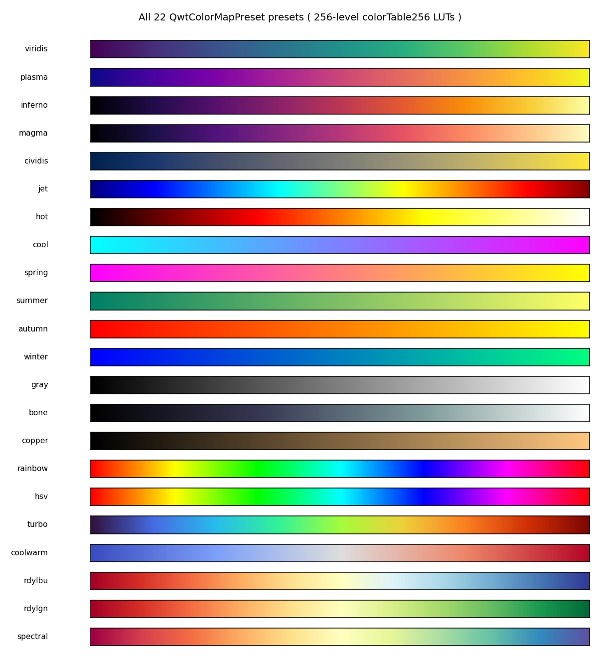
Table 1: objective classification results (stop data + LUT)

preset	class	first-last ΔE00	t(L*max)	max C*	hue sweep (°)	flag
viridis	sequential	100.32	1.000	85.82	224.1	hue sweep
plasma	sequential	109.30	1.000	91.20	159.2	-
inferno	sequential	100.82	1.000	80.91	170.4	-
magma	sequential	99.82	1.000	65.48	170.8	-
cividis	sequential	93.16	1.000	80.95	239.3	hue sweep
jet	sequential	41.51	0.627	133.81	267.7	hue sweep
hot	sequential	100.00	1.000	104.46	89.6	-
cool	sequential	57.98	0.000	115.49	131.7	-
spring	sequential	92.81	1.000	115.54	134.4	-
summer	sequential	47.38	1.000	73.26	66.2	-
autumn	sequential	64.30	1.000	104.55	62.6	-
winter	sequential	77.87	1.000	133.81	157.4	-
gray	sequential	100.00	1.000	0.00	0.0	achromatic
bone	sequential	100.00	1.000	18.66	8.3	-
copper	sequential	79.00	1.000	44.64	86.0	-
rainbow	cyclic	0.00	0.169	133.79	359.4	-
hsv	cyclic	0.00	0.169	133.79	359.4	-
turbo	sequential	30.79	0.502	94.02	282.0	hue sweep
coolwarm	diverging	40.13	0.502	70.59	191.6	-
rdylbu	diverging	37.21	0.502	77.78	281.7	hue sweep
rdylgn	diverging	63.67	0.502	77.78	129.0	-
spectral	diverging	28.86	0.502	68.77	293.6	hue sweep

The hue sweep angle accumulates only over the chromatically valid segments where C* ≥ 15 (hue angles of near-neutral colors are numerical noise); gray has C* = 0 across the whole band and bone peaks at only C* 18.66; the "hue" information of both can be ignored.

4.3 Lightness profiles and monotonicity

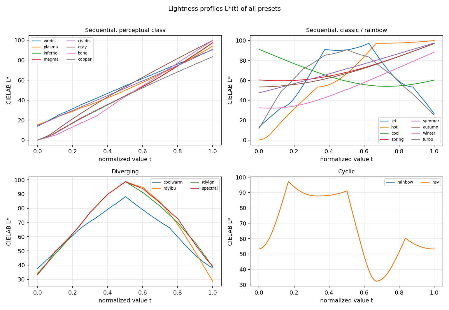
Table 2: lightness monotonicity and step uniformity (256-level LUT, normal color vision)

preset	L*₀	L*₂₅₅	viol	reg	maxreg	ΔE mean	ΔE max	CV	path	grade
viridis	14.90	90.69	0	0.02	0.02	0.482	0.948	0.294	122.98	A
plasma	15.53	93.95	0	0.00	0.00	0.482	0.970	0.427	122.92	A
inferno	0.08	97.44	0	0.00	0.00	0.590	1.596	0.364	150.43	A
magma	0.08	97.38	0	0.00	0.00	0.551	1.363	0.361	140.59	A
cividis	13.79	90.93	0	0.00	0.00	0.457	1.234	0.401	116.47	A
jet	12.97	26.47	77	71.76	70.67	0.922	1.557	0.401	235.21	C
hot	0.00	99.93	0	0.00	0.00	0.656	1.610	0.535	167.24	B
cool	91.11	60.17	0	6.31	6.24	0.312	0.431	0.362	79.49	B
spring	60.32	96.88	0	0.79	0.77	0.363	0.644	0.449	92.44	A
summer	47.49	97.45	0	0.00	0.00	0.232	0.461	0.476	59.19	B
autumn	53.24	96.88	0	0.00	0.00	0.245	0.358	0.432	62.44	A
winter	32.30	88.18	0	1.10	0.35	0.371	0.823	0.506	94.69	B
gray	0.00	99.65	0	0.00	0.00	0.294	0.398	0.228	74.96	A
bone	0.00	99.65	0	0.00	0.00	0.434	1.397	0.487	110.76	B
copper	0.00	83.44	0	0.00	0.00	0.423	1.047	0.362	107.82	A
rainbow	53.24	53.26	39	75.03	64.75	1.087	2.335	0.594	277.06	B
hsv	53.24	53.26	39	75.03	64.75	1.087	2.335	0.594	277.06	B
turbo	11.80	25.19	74	65.52	65.52	0.868	1.833	0.359	221.24	C
coolwarm	37.67	38.03	0	0.40	0.40	0.503	1.536	0.380	128.17	A
rdylbu	34.28	28.66	0	0.29	0.29	0.660	1.954	0.354	168.33	A
rdylgn	34.28	38.90	0	0.29	0.29	0.539	1.112	0.326	137.41	A
spectral	33.32	39.25	0	0.29	0.29	0.696	1.786	0.449	177.51	A

jet has the most dangerous lightness profile of all presets: L* climbs from 12.97 to 97.14 (the yellow segment at t≈0.625) and falls back to 26.47: 77 counter-direction steps, a cumulative regression of 71.76 L. The ascending branch covers [12.97, 97.14] and the descending branch covers [26.47, 97.14], so every lightness value inside (26.47, 97.14) appears at least once on each branch (up to one quantization step of error): on a grayscale or low-contrast display, two data values more than half a range apart can share the same gray. turbo has the same shape with slightly smaller magnitudes (65.52/65.52). cool is easy to miss: it decreases overall (91.11→60.17) and looks monotone, but its middle section dips to 53.94 and climbs back by 6.24 L, forming a V-shaped hollow that is invisible to the per-step tolerance and visible to the cumulative regression metric. The two arms of the four diverging presets are all well-behaved (reg ≤ 0.40): their lightness information is concentrated in the "bright center, dark arms" structure, which is read differently from a sequential ramp; mixing the two reading modes produces systematic misinterpretation.

4.4 Step uniformity

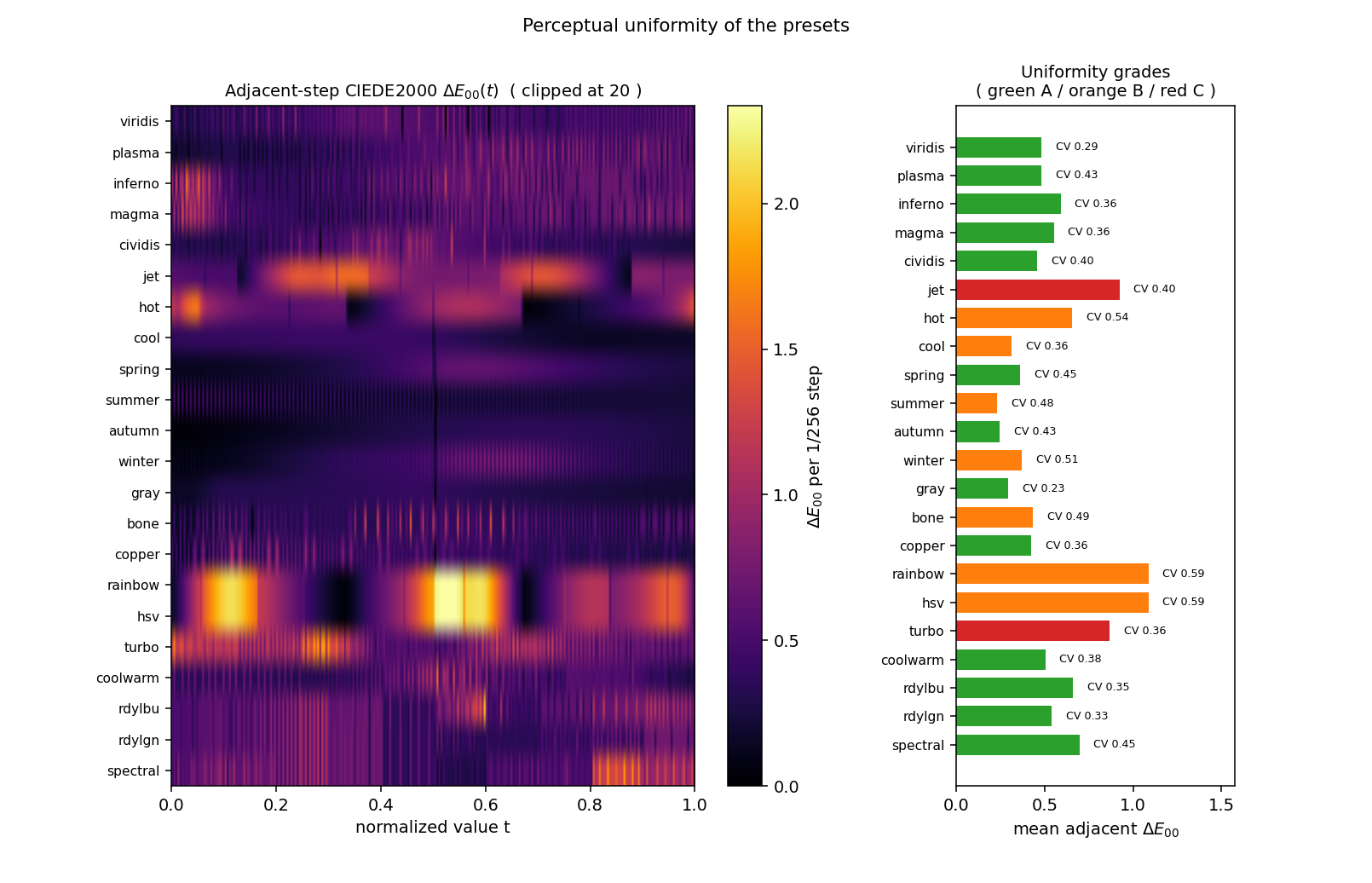
The heatmaps unfold each ramp into the sequence of its 255 adjacent-step ΔE00 values: rainbow/hsv show bright blocks with ΔE00 > 2 near the pure-hue corner points (perceptual distances between corners of the sRGB cube are far larger than between edge midpoints), and jet is likewise bright in the cyan-yellow segment; the perceptually uniform family (viridis/plasma/cividis) and the diverging family are flat overall. The CV ordering gives another view: gray is lowest at 0.228, because interpolation in the sRGB-encoded space is naturally close to perceptually uniform. The 0.364/0.361 of inferno/magma are within +0.032/+0.013 of matplotlib's own same-convention CV (inferno 0.332, magma 0.348, viridis 0.278, plasma 0.417), and viridis 0.294 is +0.016 above mpl 0.278; the remainder comes from the 9-stop linear interpolation itself. Before the fix these three presets carried CV increases of 0.136–0.255 caused by positionally compressed or deviating stops (Section 4.7); v7.5.1 resampled the stops from the official matplotlib tables. Presets with a minimum adjacent-step ΔE00 of 0.000 (viridis, cividis, summer, autumn, gray, bone, copper) contain fully duplicated LUT entries, mostly in the middle of the ramp: gray/summer/autumn/copper duplicate at level 128 (L* 44–72), the rounding pigeonhole artifact of 256 entries covering 255 output steps; viridis/cividis duplicate at levels 133–154 / 72 (L* 56–62 / 36, both mid-ramp); only bone (level 39, L* 9.3) falls at the dark end. This is quantization redundancy rather than a defect; it means these ramps lose almost no visible detail when quantized to 256 levels. Convention note: the example UI's Color Table = 256 goes through colorTable(256) (sampling grid pos = i/255), which is not the same grid as the colorTable256() pos = i/256 used here, but the conclusion is the same.

4.5 Distinguishability under color-vision deficiency

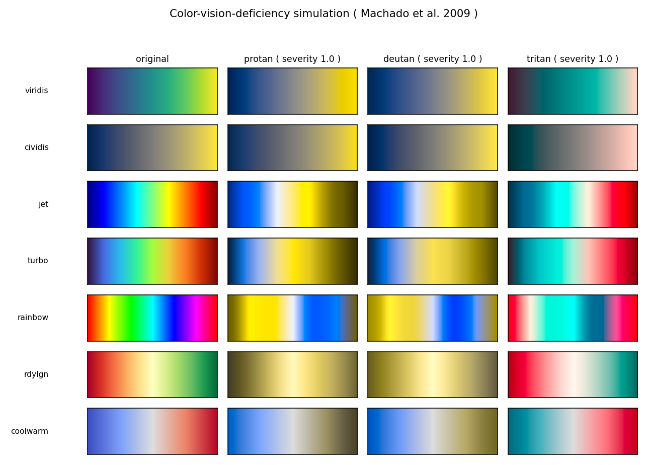
Table 3: minimum ΔE00 between levels 32 apart (farMin, distinguishability lower bound)

preset	original	protan	deutan	tritan
viridis	10.698	4.408	6.768	6.656
plasma	7.373	3.641	6.828	7.728
inferno	10.640	5.672	8.743	9.889
magma	10.043	6.077	8.744	9.337
cividis	7.004	6.844	6.957	5.849
jet	13.147	5.001	4.579	5.381
hot	4.215	2.787	3.914	1.207
cool	4.767	0.000	0.333	4.233
spring	4.404	3.133	4.844	2.513
summer	5.666	3.892	4.555	4.683
autumn	1.601	1.591	0.783	2.530
winter	2.423	1.473	1.857	1.683
gray	6.748	6.748	6.748	6.748
bone	7.648	7.566	7.373	5.012
copper	6.731	6.496	6.620	5.416
rainbow	6.529	0.297	0.130	1.198
hsv	6.529	0.297	0.130	1.198
turbo	14.979	3.931	2.268	6.136
coolwarm	10.250	10.008	9.961	10.301
rdylbu	12.487	9.632	8.866	13.237
rdylgn	8.292	1.332	0.182	10.617
spectral	6.636	1.767	0.368	6.231

Under normal vision the lowest farMin belongs to autumn (1.601): the total color path of the red-yellow ramp is only 62.44 ΔE00 (the path column of Table 2), so two points 1/8 of the range apart are separated by about 1.6 JND to begin with, a gamut choice rather than a defect. The worst cases in the deutan column (printed case by case by the script):

preset	deutan farMin	the two positions of identical color
rainbow / hsv	0.130	t = 0.620 and t = 0.745 (blue-cyan segment and blue-magenta segment)
rdylgn	0.182	t = 0.439 and t = 0.565 (the red arm and the green arm on either side of the central yellow)
cool	0.333	t = 0.616 and t = 0.741
spectral	0.368	t = 0.451 and t = 0.576
autumn	0.783	t = 0.024 and t = 0.149
winter	1.857	t = 0.004 and t = 0.129
turbo	2.268	t = 0.482 and t = 0.608

rdylgn and spectral have the most deceptive failure mode: under normal color vision they are grade-A uniform ramps, but their red and green arms collapse into the same patch of olive under deutan/protan (rdylgn, row 6 of the figure above; spectral is not in the figure, same mechanism); the sign information on either side of the center is completely lost to red-green colorblind observers. cool reaches farMin = 0.000 under protan: two levels 32 apart become strictly identical in color after simulation and 8-bit quantization, a total collision in the protan view. The cyan→magenta path carries its distinguishability on the red-green opponent axis; without that axis the simulated ramp folds back on itself and injectivity no longer holds. By contrast, coolwarm (blue-white-red) and rdylbu (red-yellow-blue) hold farMin ≥ 8.87 under all three deficiencies, because the blue-red opponent axis stays separated under protan/deutan; cividis, designed specifically for color-vision deficiency, holds farMin steady at 5.85–6.96 under all three, with no weak spot.

4.6 Grayscale-print safety

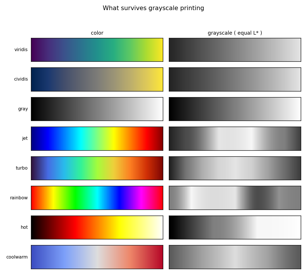
Table 4: grayscale profiles (L* is the gray level)

preset	min |ΔL*|	reg	end ΔL*	grayscale monotonic
viridis	0.0000	0.02	75.78	yes
plasma	0.0694	0.00	78.42	yes
inferno	0.0979	0.00	97.36	yes
magma	0.0791	0.00	97.30	yes
cividis	0.0000	0.00	77.14	yes
jet	0.0023	71.76	13.50	NO
hot	0.0027	0.00	99.93	yes
cool	0.0008	6.31	30.94	NO
spring	0.0008	0.79	36.56	yes
summer	0.0000	0.00	49.96	yes
autumn	0.0000	0.00	43.64	yes
winter	0.0024	1.10	55.88	yes
gray	0.0000	0.00	99.65	yes
bone	0.0000	0.00	99.65	yes
copper	0.0000	0.00	83.44	yes
rainbow	0.0011	75.03	0.01	n/a
hsv	0.0011	75.03	0.01	n/a
turbo	0.0047	65.52	13.39	NO
coolwarm	0.0723	0.40	0.36	yes
rdylbu	0.0025	0.29	5.61	yes
rdylgn	0.0980	0.29	4.62	yes
spectral	0.0869	0.29	5.93	yes

Grayscaling preserves only the information in \(L^*(t)\). Among the sequential presets, 13 of the 16 are grayscale-monotonic and can go straight to black-and-white printing; jet, turbo and cool are grayscale-non-monotonic; after printing, the bright yellow band and the dark ends create false contours (jet/turbo, rows 4 and 5 of the figure above; cool is not in the figure). The two arms of the diverging presets are each monotone, but whether the sign information survives depends on the end-to-end ΔL: coolwarm's ends differ by only 0.36 L, so in a grayscale image the positive and negative arms are exactly the same gray and the sign can only be rescued by legend text; the ends of rdylbu/rdylgn/spectral differ by 4.6–5.9 L* and the direction remains distinguishable in grayscale. Cyclic presets degrade in grayscale to gray levels oscillating back and forth (end ΔL* = 0.01), with all period information lost; cyclic data should never be carried by lightness in the first place.

4.7 Comparison against the matplotlib reference tables

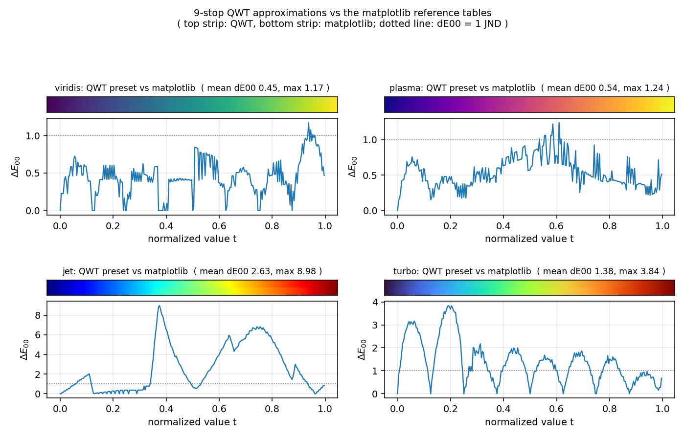
Table 5: QWT LUT vs matplotlib 256-level tables (same grid pos = i/256)

preset	mean ΔE00	max ΔE00	stop mean	stop max
viridis	0.445	1.171	0.000	0.000
plasma	0.537	1.242	0.383	0.747
inferno	1.003	3.875	0.000	0.000
magma	0.738	2.446	0.000	0.000
cividis	0.611	2.234	0.000	0.000
jet	2.634	8.978	2.613	8.978
hot	5.146	16.270	6.118	15.916
cool	0.106	0.388	0.000	0.000
spring	0.228	0.644	0.000	0.000
summer	0.118	0.392	0.000	0.000
autumn	0.162	0.358	0.000	0.000
winter	0.243	0.823	0.000	0.000
gray	0.133	0.378	0.000	0.000
bone	4.932	8.751	3.457	7.178
copper	7.918	12.509	0.000	0.000
rainbow	48.443	90.742	45.512	89.898
hsv	1.630	4.393	1.683	3.097
turbo	1.380	3.838	0.000	0.000
coolwarm	4.537	8.239	1.981	4.724
rdylbu	0.403	1.471	0.169	0.460
rdylgn	0.292	0.749	0.147	0.369
spectral	0.402	1.322	0.146	0.395

"Same name" does not mean "same colors". The provenance probe (script section 7; for every stop, a 4096-point nearest match on the matplotlib curve) yields three cases. Case one, stops lying exactly on the reference curve: all 9 stops of plasma have dE = 0.000 with nearest positions ≈ nominal positions; cool/spring/summer/autumn/winter/gray have exact first and last stops with no (or only linear) intermediate segments, whole-band deviation ≤ 0.83 (copper's first and last stops are exact too, but the mpl version is a nonlinear ramp; the whole-band mean deviation reaches 7.92, filed under item 8 of Section 5.2). Case two (removed in v7.5.1), stop colors taken from the reference curve but positions compressed: the 9 stops of inferno have nearest positions on the mpl curve at t = 0, 0.0977, 0.1993, 0.2969, 0.3985, 0.5001, 0.5978, 0.6994, 0.9963 (each dE = 0.000), the colors of the mpl curve over t∈[0,0.7] placed at positions [0,0.875], the last segment then jumping straight from t=0.7 to t=1.0; the whole band therefore has a mean deviation of 13.52 and a maximum of 28.31. turbo is approximately the same type (nearest stop-to-curve distances 0.70–2.27 ΔE00, nearest positions 0, 0.086, 0.203, 0.289, 0.391, 0.500, 0.598, 0.711, 0.996). Case three, stops deviating from the reference curve (all dE below are nearest distances to the mpl curve; same-position differences are in the "stop max" column of Table 5): the first three stops of viridis are on the curve, then drift gradually (the t=0.5 stop's nearest match is at 0.422, dE 2.62; the t=0.75 stop dE 6.52), cividis deviates by 0.77–5.82 across the band, magma deviates by ≤ 2.31 with position compression. rainbow is a different map altogether: QWT's rainbow is a closed hue loop with identical red at both ends (OpenCV style), matplotlib's rainbow is a non-closed ramp from purple to red; the mean deviation of 48.44 is a difference of definition, not of approximation error. Since v7.5.1 the five presets listed above are resampled from the official matplotlib tables: their stops sit exactly on the reference (0.000 deviation at the same position) and the whole-band mean deviation drops to viridis 0.445 / inferno 1.003 / magma 0.738 / cividis 0.611 / turbo 1.380 ΔE00, the remainder being the 9-stop linear interpolation.

Fix note (v7.5.1) — stops resampled from the official matplotlib tables

In the first release some stops were hand approximations: the 9 stops of inferno/magma/turbo were taken exactly (or nearly) from the mpl curve but placed over the whole 0-1 range (position compression), and the intermediate stops of viridis/cividis deviated from the mpl table by up to 11.4-17.2 ΔE00 at the same position. Since v7.5.1 the stops of these five presets are sampled directly from the official matplotlib 256-entry tables at the same positions (generator: colormap_stops_gen.py, rerunnable for verification): the same-position stop deviation is exactly zero and the whole-band mean deviation drops to 0.445-1.380 ΔE00 (the remainder is the 9-stop linear interpolation), and inferno/magma move from grade B to A. The other presets are unchanged: jet/hot/bone/copper/coolwarm remain few-stop approximations (item 7 of Section 5.2) and rainbow remains QWT's own closed hue ring, which never was matplotlib's same-name table.

5. Discussion

5.1 Scenario-based selection guide

Every recommendation in the table below cites measured numbers from the preceding sections.

Table 6: data type × observer × output → recommended preset

scenario	recommendation	quantitative basis
Sequential data, normal color vision, screen	viridis (or plasma)	grade A; original farMin 10.70; CV 0.294
Sequential data, red-green colorblind readers, screen	cividis	deutan farMin 6.96, protan 6.84, tritan 5.85 — no weak spot under the three deficiencies; grade A
Sequential data, dark background	inferno / magma	L*₀ = 0.08, low values blend into the background; CV 0.36, within 0.03 of the mpl tables
Sequential data, grayscale/black-and-white printing	gray (or viridis/cividis)	grayscale-monotonic with end ΔL* 75.8–99.7; jet/turbo/cool are grayscale-non-monotonic — do not use
Diverging data (signed), normal color vision, screen	coolwarm	grade A; both arms monotone, reg 0.40; farMin ≥ 9.96 under all three deficiencies
Diverging data, red-green colorblind readers	coolwarm or rdylbu	deutan farMin 9.96 / 8.87; rdylgn/spectral fall to 0.18/0.37 under deutan — do not use
Diverging data, grayscale printing	rdylbu (or rdylgn/spectral)	end ΔL* 5.61/4.62/5.93, sign distinguishable; coolwarm ends differ by ΔL* 0.36 — sign lost
Cyclic data (phase, angle), screen	rainbow / hsv	the only cyclic presets with identical ends (first-last ΔE00 = 0); accept the deutan farMin 0.13 cost, or switch to isoline/arrow encoding
Compatibility with legacy MATLAB code	jet	compatibility only; avoid in new figures: reg 71.76, grayscale-non-monotonic, deutan farMin 4.58
A rainbow look is required (compatibility scenarios)	turbo or jet, both grade C	the two trade blows on the metrics (CV 0.359 vs 0.401): turbo's lightness regression is slightly smaller (65.52 vs 71.76), jet is more distinguishable under CVD (deutan 4.58 vs 2.27); both banned for grayscale printing

Two cross-cutting recommendations. First, the color bar and the data plot must share the semantics of the same colormap instance (in the example, the spectrogram and the QwtScaleWidget each call create() once), otherwise the evaluation conclusions for the color bar do not match the plot. Second, when the readership is unknown, cividis minimizes the expected loss for sequential data: it is grade A under normal color vision (CV 0.401), has no collapse point under the three deficiencies or in grayscale, and its only cost is a hue variation more reserved than viridis's.

5.2 Failure modes

The limits of the evaluation method itself, and the negative results of this experiment, are listed below.

1. ΔE00 is insensitive to spatial frequency and area. Adjacent-step ΔE00 evaluates swatch pairs on a color bar; perception on a real plot is also shaped by region size, boundary contrast and simultaneous contrast. The same ramp reads differently in thin isolines and in large filled areas; this evaluation does not cover that.
2. The CVD matrices are a linear approximation, taken at severity 1.0 only. The Machado model is a 3×3 linear transform at the dichromacy end and ignores individual differences such as pupil, lens and macular pigment density; in real populations, anomalous trichromacy (severity 0.2–0.8) is more common than full dichromacy, and its discrimination lies between the "original" and "severity 1.0" columns above; we give only the two ends of the envelope.
3. The 256-level grid introduces quantization artifacts. Several presets have a minimum adjacent-step ΔE00 of 0.000 (duplicated entries, all in the middle of the ramp; only bone at the dark end, see Section 4.4), meaning the 8-bit grid there is already coarser than the ramp's steps; with colorTable(1024) or the continuous path, the corresponding statistics would change. farMin's gap=32 is also a convention; a different gap gives different numbers (same direction).
4. The grading thresholds are conventions, not physics. The CV 0.45/0.75 and reg 2/8 boundaries put spring and spectral (CV 0.449) almost exactly on the A/B boundary; cool's grade B comes from the distance between reg 6.31 and the threshold 8; set the threshold at 5 and it drops to C. The raw numbers in the tables are more reliable than the letters.
5. Grayscale printing is only approximated by L*. Real printing is subtractive (CMYK, paper whiteness, dot gain); the "grayscale" here is on-screen L*, an upper-bound estimate for inkjet/laser printing; presets with min |ΔL*| = 0 also accumulate halftone-dot quantization on paper.
6. The evaluation is decoupled from the data distribution. All metrics assume the data occupies the ramp uniformly over [vMin, vMax]; with skewed data or outliers, the segment of the ramp actually in play may be only a small slice of the LUT (e.g. when jet's bright band happens to cover 90% of the data, the false boundary becomes invisible instead), and the choice of vMin/vMax often matters more than the choice of ramp.
7. Deviations of the preset data from the reference implementations are counted as they are (the five mpl-sourced presets fixed in v7.5.1). In the first release QWT's viridis was not matplotlib's viridis (mean difference 6.63), so the literature's conclusion that "viridis is perceptually uniform" could not be transferred unconditionally to the stops QWT ships; since v7.5.1 viridis/inferno/magma/cividis/turbo are resampled from the official mpl tables (stop deviation 0.000, whole-band mean 0.445-1.380 ΔE00), while jet/hot/bone/copper/coolwarm remain few-stop approximations and rainbow remains QWT's own closed hue ring. Those remaining deviations are still counted, and the A/B/C grades describe the shipped QWT data only.
8. Negative results: autumn's original farMin is only 1.601 (color path too short), cool's farMin under protan is 0.000, and copper/bone deviate from mpl's same-name tables by 7.9/4.9 (both are nonlinear ramps in mpl, and a 2/4-stop linear approximation must distort; untouched by this batch); the "simple and intuitive" character of these presets is paid for in information capacity.

6. Code practice

6.1 Creating a colormap and fetching colors

#include <qwt_colormap_preset.h>

// create by name (case-insensitive; an unknown name silently falls back to viridis — spell it right)
std::unique_ptr< QwtLinearColorMap > cmap = QwtColorMapPreset::create("cividis");

// unified signature since v7.3.1+: rgb(vMin, vMax, value)
const QRgb c = cmap->rgb(0.0, 100.0, 42.0);

// query and conversion
const QStringList names = QwtColorMapPreset::availablePresets();      // 22 names
const auto stops = QwtColorMapPreset::colorStops(QwtColorMapPreset::Jet);
QwtColorMapPreset::Preset p = QwtColorMapPreset::presetFromName("TURBO");

6.2 Spectrogram + color bar

The color bar and the plot each own a colormap instance (setColorMap() transfers ownership), so create() must be called twice; the pointer cannot be shared:

#include <qwt_plot_spectrogram.h>
#include <qwt_scale_widget.h>

QwtPlotSpectrogram* spec = new QwtPlotSpectrogram();
spec->setColorMap(QwtColorMapPreset::create("coolwarm").release());
spec->attach(plot);

QwtScaleWidget* axis = plot->axisWidget(QwtAxis::YRight);
axis->setColorBarEnabled(true);
axis->setColorMap(interval, QwtColorMapPreset::create("coolwarm").release());

Warning — Ownership and NaN

setColorMap() takes ownership of the pointer; setting the same QwtColorMap* on two places causes a double free. The continuous path returns transparent black for NaN/Inf (rgb() returns 0) while the indexed path maps them to index 0; the two paths have different missing-data semantics, so mind the legend interpretation when mixing them.

6.3 Self-checks for colorblind readers and printing

Turn the metrics of Section 4 into a self-check habit at the two-lines-of-code level: export a grayscale version (or temporarily swap the colormap for gray) to check lightness monotonicity; before delivery, run diverging data with red-green opposition (rdylgn/spectral) through a deutan simulation once. Table 3 shows that a grade-A ramp under normal color vision can have a distinguishability of only 0.18 under deutan. The 3D side needs none of this repeated: Qwt3DTheme::setDataColorPreset("plasma") internally goes through the same QwtColorMapPreset factory, so the 2D evaluation conclusions apply directly.

7. Summary

Colormap evaluation reduces to three numbers: lightness monotonicity, step CV and farMin under CVD simulation. Among QWT's 22 presets, 13 are grade A under normal color vision, and the risks that decide a selection are concentrated: the lightness collapse of jet/turbo (reg 65–72 L*) rules them out wherever grayscale or low-contrast reading matters; rdylgn/spectral and the closed hue loops rainbow/hsv collapse to 0.13–0.37 ΔE00 under deutan, so sign and period information is missing for roughly 8% of male readers; coolwarm's sign information lives only in hue and is lost in grayscale print. The preset data still carries engineering debt: jet/hot/bone/copper/coolwarm remain few-stop approximations and rainbow is QWT's own closed hue ring, so "same name as matplotlib" still implies similar, not identical. The boundaries of this evaluation are equally clear: it evaluates the 256 swatches of a color bar, not perception on a real plot; it gives the envelope endpoint at severity 1.0, not the expectation over a population. Within those two boundaries, Table 6 can be used directly as a selection basis.

8. References

1. Sharma, G., Wu, W., Dalal, E. N. The CIEDE2000 color-difference formula: Implementation notes, supplementary test observations, and observations. Color Research & Application, 30(1):21-30, 2005. (includes the validation dataset; 22 pairs used in our self-test)
2. Machado, G. M., Oliveira, M. M., Fernandes, L. A. A physiologically-based model for simulation of color vision deficiency. IEEE Transactions on Visualization and Computer Graphics, 15(6):1291-1298, 2009. (severity-1.0 matrices taken from the authors' published tables)
3. Moreland, K. Diverging color maps for scientific visualization. Advances in Visual Computing, 5th International Symposium, 2009. (design criteria for diverging ramps: bright neutral center, equal perceptual weight of both arms)
4. IEC 61966-2-1:1999. Multimedia systems and equipment — Colour measurement and management — Part 2-1: Colour management — Default RGB colour space — sRGB.
5. CIE 15:2004. Colorimetry, 3rd edition. (CIELAB definition and D65 white point)
6. QWT7 sources: src/core/qwt_colormap_preset.h/.cpp (22 preset color stops), src/core/qwt_colormap.h/.cpp (QwtColorMap base class, ColorStops interpolation, colorTable256), src/plot/qwt_scale_widget.cpp (color bar), src/plot3d/qwt3d_colormap_color.h (3D bridge).
7. Experiment script: docs/assets/algorithms/colormap_experiment.py (deterministic; all raw numbers printed to stdout).
8. QWT7 example: examples/2D/colormap (interactive comparison of the 22 presets, supports --screenshot batch export).

Companion reading: Scientific Colormap Presets: usage of the 22 presets and the example UI; Raster vs OpenGL Rendering Pipelines: where colorTable256() goes in the render pipeline; NaN Rendering: the shared semantics behind rgb() returning transparent black for NaN; 3D Surface Rendering Pipeline: the other end of the Qwt3DColorMapColor bridge.