Curve Plot - QwtPlotCurve
QwtPlotCurve is the most core plot item class in Qwt, used for drawing data curves in a 2D coordinate system. It supports multiple display styles (lines, steps, sticks, etc.), symbol markers, curve fitting, and rich style configuration.
Key Features
Features
- Multiple curve styles: Lines, Steps, Sticks, Dots and other drawing modes
- Symbol marker system: Display various shapes at data points
- Curve fitting and interpolation: Built-in spline and other fitting algorithms
- High-performance rendering: Optimized rendering for large datasets
- Fill area: Configurable fill between the curve and baseline
- Legend customization: Configurable curve display style in the legend
Basic Concepts
Curve Style Types
QwtPlotCurve supports the following drawing styles:
| Style | Enum Value | Description |
|---|---|---|
| No curve | NoCurve |
Show symbols only, no connecting lines |
| Lines | Lines |
Connect data points with straight lines (default) |
| Sticks | Sticks |
Draw vertical/horizontal lines from baseline |
| Steps | Steps |
Step function style connection |
| Dots | Dots |
Draw points only (more efficient than NoCurve + Symbol) |
Curve Attribute Flags
| Attribute | Enum Value | Description |
|---|---|---|
| Inverted | Inverted |
Steps style draws from right to left |
| Fitted | Fitted |
Enable curve fitting (requires a curve fitter) |
Class Inheritance
classDiagram
class QwtPlotItem {
+attach(plot)
+setTitle()
+setRenderHint()
}
class QwtPlotSeriesItem {
+drawSeries()
+boundingRect()
+data()
}
class QwtSeriesStore~QPointF~ {
+setSamples()
+sample(i)
+size()
}
class QwtPlotCurve {
+setStyle(CurveStyle)
+setPen()
+setBrush()
+setSymbol()
+setBaseline()
+setCurveFitter()
+setCurveAttribute()
}
QwtPlotItem <|-- QwtPlotSeriesItem
QwtPlotSeriesItem <|-- QwtPlotCurve
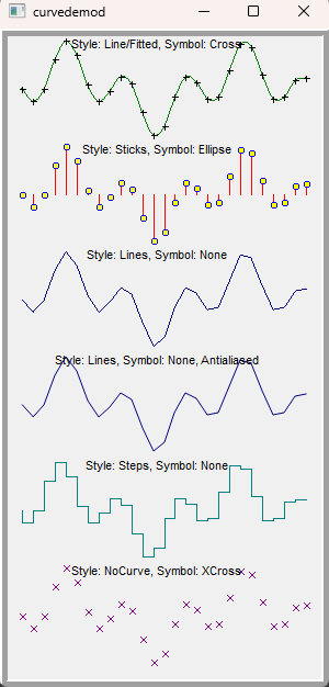
QwtSeriesStore <|-- QwtPlotCurveUsage
The curve plotting example is located at: examples/2D/curvedemo, showcasing multiple curve styles. Screenshot below:
1. Creating a Basic Curve
The most basic way to draw a curve:
1 2 3 4 5 6 7 8 9 10 11 12 13 14 15 16 17 18 19 20 21 22 23 24 25 26 27 28 29 30 31 32 | |
2. Setting Data
QwtPlotCurve provides multiple methods for setting data:
1 2 3 4 5 6 7 8 9 10 11 12 13 14 15 16 17 18 19 | |
setRawSamples Considerations
When using setRawSamples(), the curve does not copy the data but directly references the provided arrays. You must ensure:
1. The arrays remain valid for the lifetime of the curve
2. The array contents should not be modified (unless you understand the consequences)
3. Do not deallocate the arrays before the curve is destroyed
3. Curve Style Configuration
Lines Style
This is the most commonly used style, connecting data points with straight lines:
1 2 | |
Enabling the Fitted attribute allows drawing smooth curves:
1 2 3 4 5 6 7 | |
Steps Style
Step function style for displaying discrete data changes:
1 2 3 4 5 | |
Steps style comparison:
1 2 3 4 5 | |
Sticks Style
Draws vertical lines from the baseline to each data point:
1 2 3 4 5 6 7 8 9 | |
Dots Style
Draws only data points without connecting lines. This is more efficient than NoCurve + Symbol:
1 2 | |
4. Symbol Configuration
Symbols are used to display markers at each data point position:
1 2 3 4 5 6 7 8 9 10 11 12 13 14 15 16 17 18 19 | |
Common symbol shapes:
| Shape | Enum Value | Description |
|---|---|---|
| Ellipse | Ellipse |
Circle or ellipse |
| Rectangle | Rect |
Rectangle |
| Diamond | Diamond |
Diamond |
| Triangle | Triangle |
Upward triangle |
| Down Triangle | DTriangle |
Downward triangle |
| Left Triangle | LTriangle |
Left-pointing triangle |
| Right Triangle | RTriangle |
Right-pointing triangle |
| Cross | Cross |
Cross (+) shape |
| X-Cross | XCross |
X-shaped cross |
| Star | Star1 |
Six-pointed star |
| Hexagon | Hexagon |
Hexagon |
| None | NoSymbol |
No symbol displayed |
Quick symbol creation:
1 2 3 4 5 6 7 8 | |
5. Fill Area
Curves can fill the area between the baseline and data points:
1 2 3 4 5 6 7 8 9 | |
6. High-Performance Rendering
For large datasets, QwtPlotCurve provides rendering optimization attributes:
1 2 3 4 5 6 7 | |
Paint Attributes Overview
| Paint Attribute | Description |
|---|---|
ClipPolygons |
Clip polygons outside the canvas to avoid rendering invalid regions |
FilterPoints |
Filter duplicate points and points outside the canvas |
FilterPointsAggressive |
More aggressive filtering, removes intermediate points in the same pixel column |
FilterPointsPixel |
Pixel-column downsampling, keeps first/min/max/last (4 points per column) for extreme speed |
FilterPointsLTTB |
MinMax bucket downsampling (simplified LTTB), preserves waveform shape better |
MinimizeMemory |
Reduce temporary memory usage (may decrease performance) |
ImageBuffer |
Use image buffer for drawing scatter points (suitable for millions of data points) |
Default Settings
Starting from Qwt 7.x, ClipPolygons | FilterPointsAggressive is enabled by default — no manual setup needed for basic optimization.
Downsampling Algorithms in Detail
FilterPointsAggressive — Aggressive Filtering (Default)
Based on QwtPointMapper's Quad Reduce algorithm. Merges consecutive points that map to the same pixel coordinates, removing redundant intermediate points.
- Principle: Scans along both X and Y directions, reducing consecutive points mapping to the same pixel row/column to key points
- Output size: Proportional to canvas pixel dimensions, approximately
4 × max(canvas_width, canvas_height) - Best for: General large-dataset scenarios with good waveform fidelity
- Time complexity: O(n)
FilterPointsPixel — Pixel-Column Downsampling
Bins data by screen pixel columns, keeping only first/min/max/last Y values per column. Automatically uses binary search to locate the visible range for monotonically increasing X data.
- Principle: Allocates a Bin array as wide as the canvas, iterates all data points into corresponding column buckets
- Output size: At most
4 × canvas_width, completely independent of data size - Best for: Trend observation in large datasets
- Time complexity: O(n)
- Limitation: Only applicable to
Linesstyle
1 2 | |
FilterPointsPixel Caveats
This algorithm overrides FilterPointsAggressive when both are set (Pixel takes priority). Since only 4 points per column are retained, high-frequency details may be lost — suitable for trend observation rather than precise analysis.
FilterPointsLTTB — MinMax Bucket Downsampling (Recommended)
Divides the visible data range into N equal-count buckets (N = 2 × canvas width), retaining the Y-minimum and Y-maximum point from each bucket. Similar to a simplified LTTB (Largest Triangle Three Buckets) algorithm. Benchmarks show this is the fastest rendering method for million-level data.
- Principle: Splits data into equal-sized buckets by index, finds extrema in each bucket, preserves original X coordinates
- Output size: Approximately
2 × N = 4 × canvas_width - Best for: Data with uneven X distribution, scenarios requiring visual waveform preservation, and best overall performance with large datasets
- Time complexity: O(n)
- Limitation: Only applicable to
Linesstyle
1 2 | |
FilterPointsLTTB vs FilterPointsPixel
- LTTB preserves original X coordinates (not pixel-aligned), producing more accurate waveform contours
- Pixel forces all points to pixel columns — simpler implementation but not necessarily faster
- When data is too small to benefit from downsampling, LTTB automatically falls back to the Quad algorithm
- Benchmarks show LTTB outperforms Pixel on million-level data (see benchmark results below)
How to Choose a Rendering Method
Select the appropriate rendering strategy based on data scale and use case:
graph TD
    A[Data size?] -->|"< 10K points"| B[Default settings<br/>FilterPointsAggressive]
    A -->|"10K ~ 100K"| C{Need precise waveform?}
    C -->|Yes| D[FilterPointsLTTB]
    C -->|No| E[FilterPointsAggressive<br/>already enabled by default]
    A -->|"100K ~ 1M"| F{Primary goal?}
    F -->|Best performance| D
    F -->|Trend observation| G[FilterPointsPixel]
    A -->|"> 1M"| H{Display mode?}
    H -->|Best performance| D
    H -->|Scatter distribution| I["Dots style + ImageBuffer"]
    H -->|Trend observation| G
Quick Reference Table:
| Data Size | Scenario | Recommended Config | Notes |
|---|---|---|---|
| < 10K | General plotting | Default (FilterPointsAggressive) |
No extra optimization needed |
| 10K–100K | Real-time curves | FilterPointsAggressive (default) |
Default algorithm is efficient enough |
| 10K–100K | Signal analysis | FilterPointsLTTB |
Preserves waveform detail |
| 100K–1M | Real-time scrolling | FilterPointsLTTB |
Benchmarked as fastest |
| 100K–1M | Offline playback | FilterPointsLTTB |
Balances speed and waveform fidelity |
| > 1M | Trend overview | FilterPointsLTTB |
Benchmarked as fastest for million-level data |
| > 1M | Scatter distribution | Dots + ImageBuffer |
Optimized for massive scatter plots |
| > 1M | Trend observation | FilterPointsPixel |
Alternative, slightly slower than LTTB |
Usage Examples:
1 2 3 4 5 6 7 8 9 10 11 12 13 14 15 16 17 18 19 | |
Comprehensive Tips for Large Datasets
- Real-time updates: Disable
setAutoReplot(), callreplot()manually after batch updates - Monotonically increasing X data:
FilterPointsPixelandFilterPointsLTTBautomatically use binary search for visible range — no manual data trimming needed - Frequent zoom/pan scenarios:
FilterPointsLTTBis recommended, benchmarked as fastest - High-quality screenshots or exports: Temporarily disable downsampling, use
FilterPointsAggressivefor the most accurate output
Benchmark Results
Below is a real-world performance comparison with 1,000,000 data points (canvas size 680×490 px, 100 frames):
| Method | Total Time (ms) | Avg Frame Time (ms) | FPS |
|---|---|---|---|
| None (no optimization) | 26,212 | 262.12 | 3.8 |
| FilterPoints | 44,472 | 444.72 | 2.2 |
| FilterPointsAggressive (default) | 17,539 | 175.39 | 5.7 |
| FilterPointsPixel | 23,216 | 232.16 | 4.3 |
| FilterPointsLTTB | 13,349 | 133.49 | 7.5 |
Conclusions:
- FilterPointsLTTB delivers the best performance at 7.5 FPS, 32% faster than the default method
- FilterPointsAggressive is the second-best choice and is already efficient as the default
- FilterPoints basic filtering is actually the slowest — overhead exceeds benefit
- No optimization (None) is faster than FilterPoints, confirming basic filtering is counterproductive at this scale
Run Your Own Tests
You can run the examples/bench/renderbench example to benchmark rendering methods on your own hardware. The tool supports configurable data size, frame count, and waveform type, with both single-method and batch comparison modes. It generates a detailed Markdown report upon completion.
7. Legend Style Configuration
Control how the curve is displayed in the legend:
1 2 3 4 5 6 7 8 9 10 11 | |
Core Methods Summary
| Method | Description |
|---|---|
setStyle() |
Set curve style |
setPen() |
Set line pen |
setBrush() |
Set fill brush |
setSymbol() |
Set data point symbol |
setBaseline() |
Set baseline position |
setCurveAttribute() |
Set curve attributes |
setCurveFitter() |
Set curve fitter |
setPaintAttribute() |
Set rendering attributes |
setSamples() |
Set data points |
setRawSamples() |
Reference external data directly |
closestPoint() |
Find the nearest data point |
minXValue()/maxXValue() |
Get data range |
minYValue()/maxYValue() |
Get data range |
Real-Time Data Update Example
1 2 3 4 5 6 7 8 9 10 11 12 13 14 15 16 17 18 19 20 21 22 23 24 25 26 27 28 29 30 31 32 33 34 | |
Related Examples
- Curve style demo:
examples/2D/curvedemo - Simple curve:
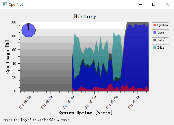
examples/2D/simpleplot - Real-time data:
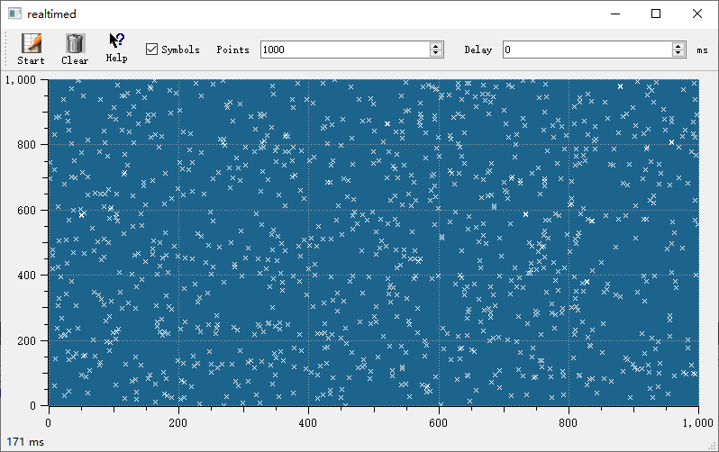
examples/2D/cpuplot - Real-time plotting:
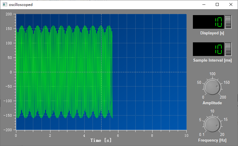
examples/2D/realtime - Oscilloscope:
examples/2D/oscilloscope
Screenshots of real-time data, real-time plotting, and oscilloscope: